Forecasting iPhone 17 Pro Demand: From Statistics to Deep LearningiPhone 需求預測:從統計模型到深度學習
An Apple Store demand forecasting problem, solved three ways—Statistics, Machine Learning, and LSTM—to explore which model truly earns its complexity.以 Apple Store 的需求規劃為例,比較統計模型、監督式機器學習與 LSTM,說明不同方法在資料規模與商業情境下的適用條件。
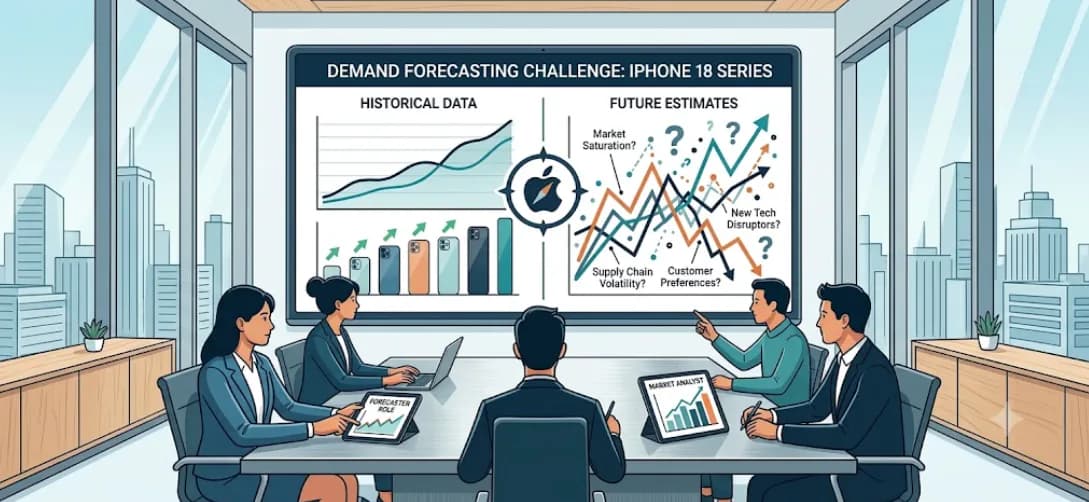
Every evening, after the Apple Store closes, a quiet but important decision takes place. The inventory system needs to answer one question:
How many iPhone 17 Pro devices should be available tomorrow?
At first glance, this sounds like a straightforward forecasting problem. In reality, it is one of the most valuable decisions in retail operations.
Forecast too low, and customers walk into the store only to discover the model they want is sold out. Some may return another day, but others may buy from another retailer or postpone their purchase entirely. Forecast too high, and expensive inventory sits in the stockroom. Unlike groceries, iPhones don't expire, but every unsold device still represents working capital that could have been invested elsewhere.
The forecast therefore influences far more than tomorrow's sales.
It drives the entire replenishment process.
Tomorrow's Demand
        ↓
Inventory Planning
        ↓
Replenishment Order
        ↓
Store Inventory
        ↓
Customer Purchase
For a single Apple Store, the financial impact may be modest. For hundreds of stores worldwide, forecasting errors quickly become millions of pounds tied up in inventory—or millions in missed revenue. The challenge is obvious.
How do we predict tomorrow's demand?
The answer has changed dramatically over the past several decades. As forecasting problems became larger and more complex, the modelling techniques evolved alongside them. In this article, we'll follow that evolution through one practical example: forecasting daily demand for the iPhone 17 Pro.
Rather than comparing algorithms in isolation, we'll see why each generation of forecasting models emerged, what business problem it solved, and when its additional complexity is actually justified.
A Typical Forecasting Problem
Let's begin with a relatively simple scenario. Suppose you're responsible for inventory planning at one Apple Store in London. Every night, you need to estimate tomorrow's demand for the iPhone 17 Pro. Fortunately, you have historical sales data from the past two years.
After plotting the data, several patterns immediately become apparent.
- Weekends are consistently busier than weekdays.
- Sales increase significantly before Christmas.
- Demand spikes immediately after new product launches.
- Demand gradually stabilises several months after launch.
- Day-to-day variation exists, but the overall behaviour is fairly predictable.
If we visualised the sales history, it might look something like this.
Demand

 ▲
 │                          Christmas
 │                           ▲
 │                           / \
 │             Launch       /   \
 │            ▲           /     \
 │            / \         /       \
 │           /   \_______/         \____
 │
 └────────────────────────────────────────► Time
As a data scientist, your first instinct might be to build a sophisticated AI model. However, experienced forecasters usually start somewhere much simpler. The first question they ask is not
"Which AI model should we use?"
Instead, they ask
"Can the historical demand already explain most of tomorrow's sales?" If the answer is yes, then a statistical forecasting model may be all we need.
Stage 1 — Statistical Forecasting
Classical forecasting begins with a simple assumption — demand is not random. Instead, it is made up of several predictable components.
For our Apple Store, those components might include
- an underlying demand level,
- a gradual trend,
- weekly seasonality,
- annual seasonality.
Rather than learning these relationships from data, statistical models describe them explicitly. One of the most widely used approaches is Holt-Winters Exponential Smoothing.
Rather than modelling the entire time series directly, Holt-Winters assumes that demand can be decomposed into several intuitive components.
Demand = Level + Trend + Seasonality
The forecasting equation
The forecasting equation can be written as
where
represents the current demand level,
represents the trend,
captures seasonal effects,
Every time new sales data arrive, these components are updated using exponential smoothing, which assigns greater weight to recent observations while gradually discounting older ones.
For our Apple Store, Holt-Winters naturally captures patterns such as
- higher weekend demand,
- increasing sales before Christmas,
- gradual changes in long-term demand.
The model is computationally inexpensive, highly interpretable, and often performs remarkably well when demand follows stable seasonal patterns.
However, Holt-Winters assumes that future behaviour can be explained by these relatively simple components. It cannot easily model more complex temporal relationships hidden within the data.
A second family of statistical models approaches forecasting from a different perspective. Instead of decomposing demand into level, trend and seasonality, ARIMA (AutoRegressive Integrated Moving Average) models how each observation depends on previous observations.
Observation
↓
Remove trend
↓
Model remaining correlations
↓
Forecast
↓
Add trend back
ARIMA makes the time series stationary by differencing — regular differencing to remove trend, seasonal differencing to remove seasonality — then model whatever autocorrelation remains in that stationary series using autoregressive (AR) and moving-average (MA) terms. It's modeling how shocks propagate and decay, not a structural level/trend/season split.
The forecasting equation
Its general formulation is ARIMA, where
is the number of autoregressive terms,
is the degree of differencing,
is the number of moving-average terms.
Conceptually, the model answers three questions.
- AutoRegressive (AR): How much does today's demand depend on previous days?
- Integrated (I): Should we remove long-term trends before modelling?
- Moving Average (MA): Can previous forecasting errors help improve future predictions?
A simplified ARIMA equation is
is the differenced series, not the raw one. tells you how many times you differenced: means (removes trend); means no differencing was needed (already stationary). This is what the "I" (integrated) in ARIMA stands for — it happens before the equation above, not inside it.
The terms (AR part, order ) say today's (differenced) value depends on its own last values: means "part of today is yesterday's value, scaled by ." means it looks back two steps, means no AR terms at all.
The terms (MA part, order ) say today also depends on the last forecast errors: means "part of today is however wrong the model was yesterday, scaled by ." This is the part that has no analog in ETS — it's explicitly correcting for recent shocks.
is a constant (drift), and is today's fresh, unpredictable shock — the part the model doesn't explain.
For example, ARIMA after differencing once:
Unlike Holt-Winters, which explicitly models trend and seasonality, ARIMA focuses on the statistical dependency between observations. For example, if demand tends to remain elevated for several days after an Apple product launch, ARIMA can capture this temporal persistence through its autoregressive component. When strong seasonal effects exist—such as increased demand every Christmas—the model can be extended to Seasonal ARIMA (SARIMA) by incorporating seasonal autoregressive and moving-average terms.
Although Holt-Winters and ARIMA take different mathematical approaches, they share the same underlying philosophy.
Historical demand contains most of the information required to forecast future demand.
This assumption is surprisingly effective for many retail forecasting problems.
Statistical models offer several important advantages.
- They require relatively little historical data.
- They train quickly on standard CPUs.
- Their predictions are highly interpretable.
- They are computationally inexpensive to deploy at scale.
- They provide strong baseline performance for products with stable demand patterns.
Even today, many supply chain forecasting systems still rely on Holt-Winters or SARIMA because they are robust, explainable, and often difficult to outperform on relatively stable products.
Stage 2 — Machine Learning
Statistical forecasting assumes that historical demand contains most of the information required to predict the future. Now imagine Apple introduces a nationwide trade-in programme for the iPhone 17 Pro. At the same time, student discounts begin, a new colour is released, and a competitor launches a flagship device.
Tomorrow's demand is now influenced by far more than historical sales alone. Neither Holt-Winters nor ARIMA naturally understands concepts such as
- promotions,
- pricing,
- holidays,
- marketing campaigns,
- competitor activity.
Their entire modelling philosophy assumes that future demand can be inferred primarily from the historical demand series.
We now need models capable of learning from multiple business variables simultaneously. This is where machine learning begins.
Instead of asking
"How can we model the demand curve?"
we now ask
"What factors influence tomorrow's demand?"
This seemingly small change marks the transition from time series modelling to supervised machine learning. Rather than modelling the demand series directly, machine learning predicts demand using a collection of explanatory variables, commonly known as features.
For our Apple Store, we might engineer features such as
Yesterday's Sales
Last Week's Sales
7-Day Moving Average
30-Day Moving Average
Weekend?
Public Holiday?
Promotion Active?
Days Since Launch
Price
Competitor Promotion
Weather
...
↓
Machine Learning Model
↓
Tomorrow's Demand
Unlike statistical models, machine learning is no longer limited to historical demand alone. Every feature represents another piece of information that may help explain customer purchasing behaviour.
The simplest machine learning model is Linear Regression. Instead of assuming demand consists of level, trend and seasonality, regression assumes that tomorrow's demand is a weighted combination of multiple explanatory variables.
The forecasting equation
The model can be written as
where
- = yesterday's sales,
- = weekend indicator,
- = promotion,
- = product price,
- = days since launch,
and each coefficient represents how strongly that feature influences future demand.
For example, the model may learn that running a promotion increases expected daily sales by 35 units, while weekends contribute an additional 20 units on average.
This is a major step beyond ARIMA. Statistical models primarily learn patterns within the demand series. Regression learns relationships between demand and business variables.
However, it comes with one important assumption - the relationships are approximately linear. Unfortunately, retail demand rarely behaves that way.
Tree-based models, such as Random Forest, XGBoost, and LightGBM, go a step further. They automatically discover nonlinear interactions—for example, a promotion might have a much larger impact during the first month after launch than six months later, or weekend demand might only increase significantly when a promotion is active. This flexibility makes tree-based models particularly attractive for retail forecasting because they naturally combine many different business signals without requiring complex mathematical assumptions.
Imagine Apple launches a promotion. Will demand always increase by the same amount?
Probably not.
A promotion during Black Friday may generate far more demand than the exact same promotion in February.
Likewise, a student discount may have little impact immediately after a product launch, but become highly effective six months later. These interactions are difficult to capture using a single linear equation.
Decision trees solve this problem differently. Instead of fitting one mathematical equation, they repeatedly divide the data into increasingly similar groups.
Conceptually, the model asks a sequence of questions.
                    Promotion?
                        │
                   Yes / \ No
                     ▼   ▼

                Weekend?
                     │ Forecast = 45
                Yes / \ No
                  ▼   ▼
      Forecast = 120   Forecast = 80
Rather than estimating coefficients, the model learns a hierarchy of decision rules. For our Apple Store, it might discover patterns such as promotions matter much more on weekends, high prices reduce demand only after launch demand subsides, Black Friday behaves differently from ordinary weekends.
These nonlinear interactions are discovered automatically without requiring us to specify them in advance.
Although a single decision tree is easy to interpret, it is rarely accurate enough for production forecasting.
Modern retail forecasting systems therefore rely on ensemble methods, particularly Gradient Boosting, with algorithms such as XGBoost and LightGBM becoming industry standards.
Instead of building one complex tree, gradient boosting builds many small trees sequentially. Each new tree focuses on correcting the forecasting errors made by the previous trees. The final prediction is simply the sum of all individual trees.
The forecasting equation
The model can be written as
where
- = represents the prediction from the (m)-th tree,,
- = is the total number of trees.
Conceptually, the learning process looks like this.
Tree 1
↓
Residual Errors
↓
Tree 2
↓
Residual Errors
↓
Tree 3
↓
...
↓
Final Forecast
Rather than trying to build one perfect model, gradient boosting gradually improves the forecast by learning from previous mistakes. This simple idea has proven extraordinarily effective.
For tabular business data, algorithms such as XGBoost and LightGBM continue to outperform many deep learning models while remaining relatively fast and interpretable.
Stage 3 — Deep Learning
Machine learning represented a major leap beyond traditional statistical forecasting. It could combine historical demand with promotions, pricing, holidays, marketing campaigns and many other business signals simultaneously.
However, despite their impressive predictive power, these models shared one important limitation — Feature engineering.
Before training could even begin, data scientists first had to decide which historical information might be useful. For example,
lag_1
lag_7
lag_14
lag_28
rolling_mean_7
rolling_std_30
days_since_launch
promotion_flag
holiday_flag
...
These features were not learned by the model. They were manually designed by engineers. As the number of products and stores grew into the thousands, maintaining hundreds of handcrafted features quickly became one of the most time-consuming parts of the forecasting pipeline.
Naturally, researchers began asking a new question.
Can the model learn these temporal representations directly from the raw demand sequence, without requiring manual feature engineering?
Learning from Sequences Instead of Features
Rather than feeding engineered variables into the model, an LSTM receives the historical demand sequence directly.
Historical Demand
↓
LSTM
↓
Tomorrow's Demand
Instead of explicitly telling the model to use a 7-day moving average or a 28-day lag, the network learns which historical observations matter during training.
This process is known as representation learning.
Rather than learning from handcrafted features, the model learns its own internal representation of demand dynamics.
Conceptually, every day's sales update an internal memory.
Day 1
↓
Memory
↓
Day 2
↓
Updated Memory
↓
Day 3
↓
Updated Memory
↓
...
↓
Forecast
Unlike traditional neural networks, which process every observation independently, an LSTM carries information forward through time using a hidden state. This hidden state acts as the model's memory, allowing information from previous days to influence future predictions
Why Ordinary RNNs Weren't Enough Early recurrent neural networks (RNNs) already processed sequential data. Unfortunately, they struggled to remember information over long periods.
As each new observation arrived, information from earlier timesteps gradually weakened during training, a problem known as the vanishing gradient. For demand forecasting, this is a serious limitation.
Imagine today's sales are influenced by
- a product launch three weeks ago,
- a promotion that started last Friday,
- Christmas approaching next month.
A vanilla RNN often struggles to retain all of these signals simultaneously.
LSTM was specifically designed to overcome this problem. The key innovation of an LSTM is its memory cell. Instead of blindly passing information forward, the network continuously decides
- what information should be remembered,
- what information should be forgotten, and
- what information should influence the next prediction.
The forecasting equation
Mathematically, an LSTM is controlled by three gates.
The forget gate determines how much of the previous memory should be retained.
The input gate decides what new information should be written into memory.
Finally, the output gate controls which parts of the memory are used to produce the next hidden state and prediction.
Although these equations appear more complicated than regression or ARIMA, their intuition is surprisingly simple.
Instead of manually creating lag features, the network gradually learns which historical information deserves to remain in memory.
At first glance, LSTMs seem strictly better than traditional machine learning. After all, they automatically discover temporal features while eliminating manual feature engineering. In practice, however, they introduce a different challenge.
They require a tremendous amount of data.
Our Apple Store sells only one product.
Even with two years of daily sales, we have roughly
365 × 2
≈ 730 observations
This is a tiny dataset for a neural network containing thousands of trainable parameters. Under these conditions, an XGBoost model with carefully engineered features will often outperform an LSTM. The deep learning model simply does not have enough examples to learn robust temporal representations.
When Deep Learning Finally Wins?
Now imagine Apple no longer forecasts demand for a single product in a single store.
Instead, it forecasts
- hundreds of products,
- across hundreds of stores,
- over many years of sales history.
500 Stores
×
300 Products
×
5 Years

↓
Millions of Historical Observations
↓
One Global LSTM
The problem has fundamentally changed.
Although each individual store may contain only a few years of data, the combined dataset contains millions of observations. The network can now learn patterns that generalise across the entire retail network.
For example,
- weekend purchasing behaviour,
- launch demand curves,
- promotional uplift,
- seasonal shopping patterns,
- inventory replenishment cycles.
Knowledge learned from one Apple Store can improve forecasts for another.
This ability to share statistical strength across many related time series is one of the primary reasons deep learning has become increasingly successful in large-scale retail forecasting.
Choosing the Right Tool
One of the biggest misconceptions in forecasting is that newer models automatically produce better forecasts.
They don't.
Each generation of forecasting models emerged because the business problem became more difficult.
| Business Problem | Suitable Approach | Why |
|---|---|---|
| One product, one store, stable demand | Statistical forecasting | Simple, interpretable, little data required |
| Rich business signals (price, promotions, holidays) | Regression or tree-based machine learning | Learns relationships between many business variables |
| Hundreds of stores and products | Global LSTM | Learns shared temporal patterns across many related time series |
The question is therefore not
"Which model is the most advanced?"
Instead, ask
"How much information do I have, and how complex is the forecasting problem?"
The best forecasting model is the one whose complexity is justified by the business—not the one with the most sophisticated architecture. Good supply chain forecasting has never been about building the smartest AI. It has always been about making better inventory decisions.
每天晚上,Apple Store 打烊後,庫存系統都必須回答一個重要問題:
明天應該備多少台 iPhone 17 Pro?
這看似只是預測問題,實際上卻直接影響零售營運的庫存成本與銷售機會。
預測太低,顧客走進店裡才發現想要的型號已經賣完。有些人可能改天再來,但也有人會轉向其他通路購買,或乾脆延後購買。 預測太高,昂貴的庫存就會堆在後場。iPhone 不像生鮮食品會過期,但每一台賣不出去的手機,都代表一筆原本可以投入其他用途的營運資金。
因此,這個預測影響的遠不只是明天的銷售量。
它牽動著整個補貨流程。
明日需求
        ↓
庫存規劃
        ↓
補貨訂單
        ↓
門市庫存
        ↓
顧客購買
對單一門市而言,每日誤差的影響或許有限;但擴大到數百家門市與多種產品配置後,小幅誤差也可能累積成可觀的庫存占用或銷售損失。
我們該如何預測明天的需求?
過去數十年,隨著資料規模與預測情境日益複雜,處理這個問題的方法也持續演進。本文透過虛構的 iPhone 17 Pro 每日需求案例,說明三個主要階段。
重點不只是比較演算法,而是理解每類模型解決了什麼問題,以及增加的複雜度在什麼條件下才具有實際價值。
一個典型的預測問題
先從一個相對單純的情境開始。假設你負責倫敦一家 Apple Store 的庫存規劃。 每天晚上,你都得估計明天 iPhone 17 Pro 的需求。幸運的是,你手上有過去兩年的歷史銷售資料。
把資料畫出來之後,幾個模式立刻浮現。
- 週末的銷售量一貫比平日高。
- 聖誕節前銷售會明顯上升。
- 新品剛上市時,需求會立刻暴增。
- 上市幾個月後,需求會逐漸趨於穩定。
- 每天的波動確實存在,但整體行為相當可預測。
如果把銷售歷史畫成圖,大概會長這樣。
需求

 ▲
 │                          聖誕節
 │                           ▲
 │                           / \
 │             上市         /   \
 │            ▲           /     \
 │            / \         /       \
 │           /   \_______/         \____
 │
 └────────────────────────────────────────► 時間
第一個問題通常不應是:
「我們該用哪一種 AI 模型?」
而應是:
「歷史需求本身,是否已經能解釋明天大部分的銷售?」
如果答案是肯定的,那麼一個統計預測模型可能就已經足夠。
第一階段 — 統計預測
傳統預測方法通常假設,需求可以分解為若干具有結構的成分,而不只是完全隨機的波動。
以我們的 Apple Store 為例,這些成分可能包括
- 一個基礎需求水準,
- 一個緩慢變化的趨勢,
- 每週季節性,
- 年度季節性。
統計模型會以預先定義的結構表示這些關係,再從資料估計各項參數。 其中最廣泛使用的方法之一,是 Holt-Winters 指數平滑法。
Holt-Winters 以水準、趨勢與季節性狀態表示時間序列。
需求 = 水準 + 趨勢 + 季節性
預測公式
預測方程式可以寫成
其中
代表目前的需求水準,
代表趨勢,
捕捉季節效應, 是季節週期, 是預測步數。
每當有新的銷售資料進來,這些成分都會透過指數平滑法更新——愈近期的觀測值權重愈高,愈久遠的觀測值權重則逐漸降低。
對我們的 Apple Store 而言,Holt-Winters 能自然捕捉到以下模式
- 週末需求較高,
- 聖誕節前銷售上升,
- 長期需求的緩慢變化。
這個模型運算成本低、高度可解釋,而且當需求呈現穩定的季節模式時,表現往往相當出色。
然而,Holt-Winters 假設未來的行為可以用這些相對簡單的成分解釋。它難以捕捉資料中隱藏的、更複雜的時間關係。
另一類統計模型則從不同角度處理預測問題。 ARIMA(自迴歸整合移動平均模型) 不將需求拆解成水準、趨勢與季節性,而是對每個觀測值如何依賴先前的觀測值進行建模。
觀測值
↓
移除趨勢
↓
對剩餘的相關性建模
↓
預測
↓
加回趨勢
ARIMA 透過差分讓時間序列變得平穩——用一般差分移除趨勢,用季節差分移除季節性——接著用自迴歸(AR)與移動平均(MA)項,對這個平穩序列中剩餘的自我相關性建模。 它建模的是衝擊如何傳播與衰減,而不是像水準/趨勢/季節那樣的結構性拆解。
預測公式
它的一般形式是 ARIMA,其中
是自迴歸項的數量,
是差分的階數,
是移動平均項的數量。
從概念上來說,這個模型在回答三個問題。
- 自迴歸(AR):今天的需求,有多少取決於前幾天?
- 整合(I):建模之前,是否需要先移除長期趨勢?
- 移動平均(MA):先前的預測誤差,能不能幫助改善未來的預測?
一個簡化版的 ARIMA 方程式是
是差分後的序列, 則是原始序列。 代表差分階數: 使用一階差分 ; 則直接對原始序列建模。這就是 ARIMA 中「I」(整合)的含義。
項(AR 部分,階數為 )代表今天(差分後)的值,取決於自己過去 個值: 的意思是「今天的一部分,是昨天的值乘上 這個係數」。 表示往回看兩步, 則代表完全沒有 AR 項。
項(MA 部分,階數為 )代表今天也取決於過去 個預測誤差: 的意思是「今天的一部分,是昨天模型犯錯的程度乘上 」。這部分在 ETS 中沒有對應的概念——它明確地在修正近期的衝擊。
是常數項(漂移), 則是今天全新、無法預測的衝擊——也就是模型無法解釋的部分。
舉例來說,差分一次之後的 ARIMA:
與明確建模趨勢和季節性的 Holt-Winters 不同,ARIMA 關注的是觀測值之間的統計相依性。 舉例來說,如果 Apple 產品上市後,需求往往會持續偏高好幾天,ARIMA 就能透過它的自迴歸成分,捕捉到這種時間上的持續性。 當存在強烈的季節效應時——例如每年聖誕節需求都會上升——這個模型可以延伸成 季節性 ARIMA(SARIMA),加入季節性的自迴歸與移動平均項。
雖然 Holt-Winters 與 ARIMA 採取不同的數學路徑,但它們背後的哲學是一致的。
歷史需求已經包含了預測未來需求所需的大部分資訊。
這個假設,對許多零售預測問題來說,效果出乎意料地好。
統計模型有幾個重要優點。
- 只需要相對少量的歷史資料。
- 在一般 CPU 上就能快速訓練。
- 預測結果高度可解釋。
- 大規模部署的運算成本低。
- 對需求模式穩定的商品,能提供具競爭力的基準表現。
直到今天,許多供應鏈預測系統仍然仰賴 Holt-Winters 或 SARIMA,因為它們穩健、可解釋,而且在相對穩定的商品上,往往很難被超越。
第二階段 — 機器學習
統計預測假設歷史需求已經包含了預測未來所需的大部分資訊。 現在想像 Apple 推出全國性的 iPhone 17 Pro 以舊換新方案。與此同時,學生優惠開始實施、新色系推出,而競爭對手也發表了旗艦機種。
此時,明日需求不再只由歷史銷售決定。若未另外加入外生變數,Holt-Winters 與標準 ARIMA 無法直接納入:
- 促銷活動,
- 定價,
- 假期,
- 行銷活動,
- 競爭對手動態。
它們整套建模哲學,都假設未來需求主要可以從歷史需求序列推得。
我們現在需要能同時從多個商業變數學習的模型。 這正是監督式機器學習適合介入的情境。
問題不再是
「我們該如何為需求曲線建模?」
而是變成
「哪些因素影響了明天的需求?」
這個看似微小的轉變,標誌著從時間序列建模轉向 監督式機器學習。 機器學習不直接對需求序列建模,而是用一組解釋變數——也就是常說的 特徵(features)——來預測需求。
以我們的 Apple Store 為例,我們可能會設計以下特徵
昨日銷售量
上週銷售量
7 天移動平均
30 天移動平均
是否為週末?
是否為國定假日?
是否有促銷活動?
距離上市天數
價格
競爭對手促銷
天氣
...
↓
機器學習模型
↓
明日需求
監督式模型可以同時使用需求歷史與外部特徵,每個特徵都代表一項可能有助於解釋購買行為的資訊。
最簡單的機器學習模型是 線性迴歸(Linear Regression)。 迴歸模型不假設需求由水準、趨勢與季節性組成,而是假設明天的需求,是多個解釋變數的加權組合。
預測公式
這個模型可以寫成
其中
- = 昨日銷售量,
- = 是否為週末,
- = 是否有促銷,
- = 產品價格,
- = 距離上市天數,
而每個係數 ,代表該特徵對未來需求的影響有多強。
舉例來說,模型可能會學到促銷活動平均能讓每日預期銷售量增加 35 台,而週末平均能再貢獻 20 台。
這是超越 ARIMA 的重要一步。統計模型主要學習需求序列本身的模式, 迴歸模型則學習需求與商業變數之間的關係。
不過,線性迴歸假設這些影響能以線性、可加的方式表示,而零售需求往往包含門檻與交互作用。
樹模型(tree-based models),例如 Random Forest、XGBoost 與 LightGBM,則更進一步。它們能自動發現非線性的交互作用——例如促銷活動在上市第一個月的效果,可能遠大於六個月後;又或者週末需求,可能只有在促銷同時進行時才會明顯上升。 這種彈性,讓樹模型在零售預測中特別受歡迎,因為它們能自然地結合許多不同的商業訊號,而不需要複雜的數學假設。
想像 Apple 推出一項促銷活動。 需求每次都會增加同樣的幅度嗎?
大概不會。
黑色星期五期間的促銷,帶來的需求可能遠大於二月同一項促銷。
同樣地,學生優惠在產品剛上市時可能幾乎沒有效果,但六個月後卻可能變得非常有效。 這些交互作用,很難用單一線性方程式捕捉。
決策樹(decision trees) 用不同的方式解決這個問題。 它不是去擬合一個數學方程式,而是不斷把資料切分成愈來愈相似的群組。
從概念上來說,這個模型是在依序提出一連串問題。
                    是否促銷?
                        │
                    是 / \ 否
                     ▼  ▼

                是否週末?
                      │ 預測 = 45
                  是 / \ 否
                   ▼  ▼
            預測 = 120   預測 = 80
這個模型學到的不是係數,而是一套階層式的決策規則。 以我們的 Apple Store 為例,它可能會發現這樣的模式:促銷活動在週末的效果重要得多;高價只有在上市熱潮退去後才會壓低需求;黑色星期五的行為,和一般週末並不相同。
這些非線性的交互作用,是模型自動發現的,不需要我們事先指定。
雖然單一決策樹較容易解釋,但預測表現通常不如經過適當正則化的集成模型穩定。
因此,現代零售預測系統大多仰賴集成方法(ensemble methods),特別是 梯度提升(Gradient Boosting),其中 XGBoost 與 LightGBM 等演算法,已經成為業界標準。
梯度提升不是建立一棵複雜的樹,而是依序建立許多小樹。 每一棵新的樹,都專注於修正前面所有樹合起來所犯的預測誤差。 最終的預測,就是所有個別樹的總和。
預測公式
這個模型可以寫成
其中
- = 第 棵樹的預測值,
- = 樹的總數。
從概念上來說,這個學習過程大致如下。
第 1 棵樹
↓
殘差
↓
第 2 棵樹
↓
殘差
↓
第 3 棵樹
↓
...
↓
最終預測
梯度提升不是試圖一次打造出完美的模型,而是透過不斷從先前的錯誤中學習,逐步改善預測。 這種逐步修正誤差的方式,在許多表格型資料問題上相當有效。
對許多表格型商業資料而言,XGBoost 與 LightGBM 仍是具競爭力的基準,通常具備訓練快速、能處理非線性關係,且可搭配特徵歸因工具等優點。
第三階段 — 深度學習
機器學習,是超越傳統統計預測的一大躍進。 它能同時結合歷史需求、促銷、定價、假期、行銷活動,以及許多其他商業訊號。
不過,這類模型普遍依賴一項重要工作:特徵工程(feature engineering)。
在訓練開始之前,資料科學家必須先決定哪些歷史資訊可能有用。 例如:
lag_1
lag_7
lag_14
lag_28
rolling_mean_7
rolling_std_30
days_since_launch
promotion_flag
holiday_flag
...
這些特徵由建模者事先設計,而不是模型直接從原始序列學習。當商品與門市規模擴大時,建立、驗證與維護大量手工特徵會成為預測系統的重要成本。
很自然地,研究者開始問一個新問題。
模型能不能直接從原始需求序列中,學到這些時間表徵,而不需要人工做特徵工程?
從序列而非特徵中學習
LSTM 不是把工程師設計好的變數餵給模型,而是直接接收歷史需求序列。
歷史需求
↓
LSTM
↓
明日需求
建模者不必明確指定 7 天移動平均或 28 天落後值;網路會根據訓練目標,學習如何組合歷史觀測值。
這個過程稱為 表徵學習(representation learning)。
模型學到的不是手工打造的特徵,而是它自己對需求動態的內部表徵。
從概念上來說,每一天的銷售都會更新一個內部記憶。
第 1 天
↓
記憶
↓
第 2 天
↓
更新後的記憶
↓
第 3 天
↓
更新後的記憶
↓
...
↓
預測
傳統神經網路獨立處理每一筆觀測值,LSTM 則不同:它透過一個隱藏狀態(hidden state),把資訊隨著時間往前傳遞。 這個隱藏狀態,就像模型的記憶,讓過去幾天的資訊,能持續影響未來的預測。
為什麼一般 RNN 還不夠 早期的循環神經網路(RNN)其實已經能處理序列資料,可惜的是,它們很難記住長期以前的資訊。
隨著新觀測值不斷進來,訓練過程中,較早期時間點的資訊會逐漸減弱,這個問題稱為 梯度消失(vanishing gradient)。 對需求預測而言,這是一個嚴重的限制。
想像今天的銷售,同時受到以下因素影響:
- 三週前的產品上市,
- 上週五開始的促銷活動,
- 下個月即將到來的聖誕節。
一般的 RNN,往往很難同時保留這些訊號。
LSTM 正是為了解決這個問題而設計的。 LSTM 的關鍵創新在於它的記憶單元(memory cell)。網路不會盲目地把資訊往前傳遞,而是持續決定
- 哪些資訊應該被記住,
- 哪些資訊應該被遺忘,
- 哪些資訊應該影響下一次的預測。
預測公式
數學上,LSTM 由三個閘門控制。
遺忘閘(forget gate)決定要保留多少先前的記憶。
輸入閘(input gate)決定哪些新資訊應該寫入記憶。
最後,輸出閘(output gate)決定記憶中的哪些部分,會被用來產生下一個隱藏狀態與預測值。
雖然這些方程式看起來比迴歸或 ARIMA 複雜,但背後的直覺其實相當簡單。
網路不需要人工建立落後期(lag)特徵,而是逐漸自己學會哪些歷史資訊值得留在記憶中。
乍看之下,LSTM 似乎完全優於傳統機器學習。 畢竟它能自動發現時間特徵,還省去了人工特徵工程。 但實際上,它帶來的是另一種挑戰。
它通常需要更多資料。
我們的 Apple Store 只銷售一項產品。
就算有兩年的每日銷售資料,也大約只有
365 × 2
≈ 730 筆觀測值
對具有數千個可訓練參數的神經網路而言,這個資料集很小。在這種情況下,具備良好特徵的 XGBoost 往往更容易訓練,也可能優於 LSTM;實際結果仍應透過依時間順序的回測確認。
深度學習何時才真正勝出?
現在想像 Apple 不再只預測單一門市、單一產品的需求。
而是要預測
- 數百項產品,
- 遍布數百家門市,
- 橫跨多年的銷售歷史。
500 家門市
×
300 項產品
×
5 年

↓
數百萬筆歷史觀測值
↓
一個全域 LSTM
此時,問題已從單一序列預測轉為跨序列的全域建模。
雖然每一家門市個別來看,可能只有幾年的資料,但把所有門市加總起來,整個資料集卻包含數百萬筆觀測值。 此時,網路就能學到能夠橫跨整個零售網路、具有一般化能力的模式。
例如:
- 週末購買行為,
- 新品上市後的需求曲線,
- 促銷帶來的提升效果,
- 季節性購物模式,
- 庫存補貨週期。
從某家門市學到的共享模式,可能改善其他相關門市的預測。
這種能在許多相關時間序列之間共享統計資訊的能力,正是深度學習在大規模零售預測中愈來愈成功的主要原因之一。
選擇合適的工具
預測工作常見的誤解,是認為較新的模型必然帶來更好的結果。
事實並非如此。
每一代預測模型的出現,都是因為商業問題本身變得更困難。
| 商業問題 | 合適的方法 | 原因 |
|---|---|---|
| 單一產品、單一門市、需求穩定 | 統計預測 | 簡單、可解釋、所需資料量少 |
| 豐富的商業訊號(價格、促銷、假期) | 迴歸或以樹為基礎的機器學習 | 能學習多個商業變數之間的關係 |
| 數百家門市與產品 | 全域 LSTM | 能跨多條相關時間序列,學習共享的時間模式 |
因此,真正該問的問題不是
「哪一個模型最先進?」
而是
「我手上有多少資訊,這個預測問題又有多複雜?」
合適的預測模型,應以足以滿足商業需求的最低合理複雜度為原則,而不是追求最複雜的架構。供應鏈預測的最終目的,是改善庫存與補貨決策。