Demand Forecasting with Statistical Models: How Far Can Demand History Alone Take Us?僅憑歷史需求,能把需求預測做到多準?
A practical and theoretical guide to forecasting iPhone demand with Holt–Winters and SARIMA—from backtesting and model selection to point forecasts.以 iPhone 隔日需求為例,實作 Holt–Winters 與 SARIMA,完整說明時間序列回測、模型選擇、殘差診斷與預測區間。
This is the statistical deep dive behind Forecasting iPhone 17 Pro Demand: From Statistics to Deep Learning. The broader article compares three generations of forecasting models. Here, we slow down and ask a narrower question:
How much of tomorrow's demand can we forecast from demand history alone?
The answer establishes a baseline that every more complex model must beat.
This article is structured as follows:
- The decision behind the forecast
- One series, several behaviours
- Forward-walking backtesting
- Traditional statistical time-series forecasting
- How do we choose parameters?
- Evaluation metrics and model selection
- From point forecast to a 95% prediction interval
- Recommendation for inventory decision
The decision behind the forecast
Every evening, the inventory team in a synthetic London Central Apple Store scenario must decide how many units of one configuration—iPhone 17 Pro 256GB Light—should be available the following day.
Forecast too low and the store risks stockouts, lost sales, and disappointed customers. Forecast too high and expensive devices occupy working capital and storage capacity. At one store, the difference may look modest. Across many stores and configurations, small daily errors accumulate into a material inventory decision.
The modelling target is therefore:
and the operational question is:
How many units should be positioned before tomorrow begins?
A demand forecast does not automatically tell us how many phones to stock. That decision also depends on the cost of having too few phones compared with the cost of having too many. If stockouts are more expensive, the planner should choose a higher point in the forecast distribution. If excess inventory is more expensive, the planner should choose a lower point. The newsvendor model expresses this choice as:
Here, is the cost of understocking, is the cost of overstocking, selects the corresponding quantile from the forecast demand distribution, and is the recommended inventory quantity. Because these costs are not available in this experiment, we cannot calculate an optimal inventory quantile. We therefore report the point forecast and 95% prediction interval as forecasting outputs, leaving the service-level decision to the business.
One series, several behaviours
The synthetic dataset contains 730 simulated daily observations from 19 September 2025 to 18 September 2027. Mean demand is 39.5 units per day. The model receives only the date and historical unit demand for this store-SKU combination.
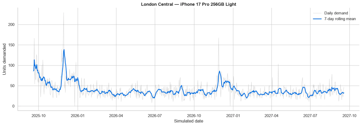
Daily observations are shown in grey; the seven-day rolling mean exposes the slower movement in demand.
The chart contains several distinct forms of temporal structure:
- Lifecycle: demand begins high after launch and declines toward a more mature level.
- Weekly seasonality: the day of the week changes the expected demand.
- Calendar effects: Christmas creates sharp local peaks, while closure days can produce genuine zero demand.
- Level changes: the local baseline rises and falls rather than remaining constant across two years.
- Irregular shocks: promotions and other commercial events produce spikes that are not explained by trend or weekday alone.
This is a univariate forecasting problem: the history of is the entire information set. Price, promotions, marketing, holidays, weather, and competitor activity are deliberately withheld. Their effects appear only after they reach the series as unexplained demand shocks.
That constraint is useful. Before giving a machine-learning model more features, we first want to know what the demand series can explain by itself.
Forward-walking backtesting
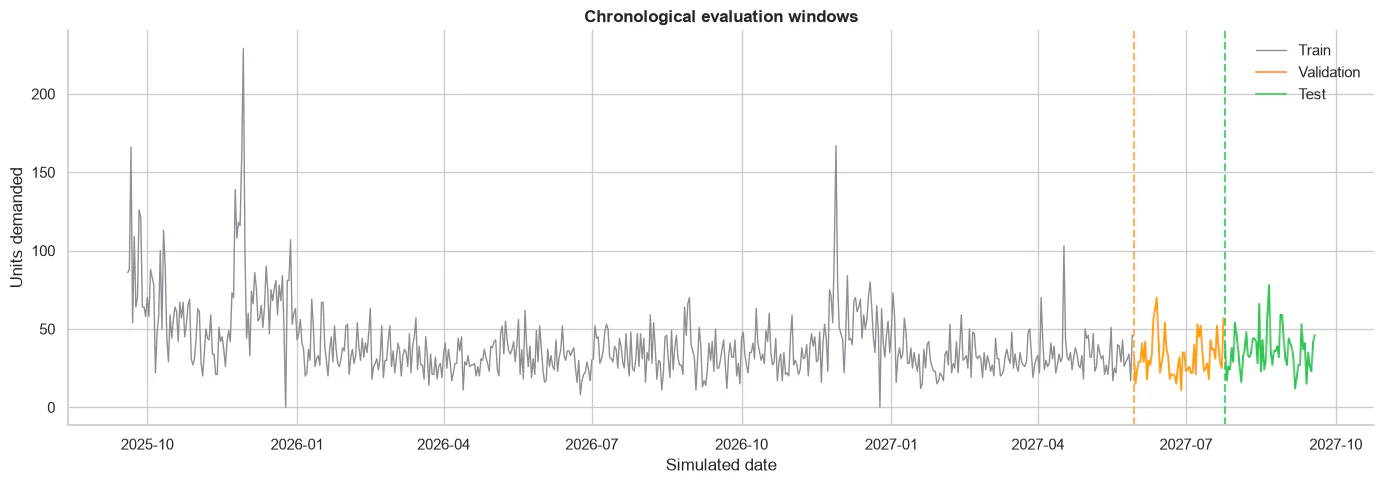
A random train-test split would leak future market conditions into the past. Instead, the observations are divided chronologically:
| Window | Observations | Dates | Purpose |
|---|---|---|---|
| Training | 618 | 19 Sep 2025–29 May 2027 | Fit candidate models |
| Validation | 56 | 30 May–24 Jul 2027 | Select one specification per family |
| Test | 56 | 25 Jul–18 Sep 2027 | Estimate final performance once |
The evaluation then reproduces the nightly workflow:
- Fit the model using every observation available at the end of day .
- Forecast demand for day .
- Reveal the actual demand for .
- Add that observation to the available history.
- Move forward one day and repeat.
This is variously called walk-forward validation, rolling-origin evaluation, or time-series backtesting. The forecast horizon remains one day, while the forecast origin advances through the validation and test windows.
At each step, the models use only observations available at that point in time. Candidate specifications are selected on the validation window and then locked before evaluation on the test window. This prevents the test data from influencing model design and keeps the reported performance realistic.
Traditional statistical time-series forecasting
Both Holt–Winters and ARIMA assume that the series' own history contains useful information about its future. They differ in what they believe that information looks like.
Holt–Winters: forecast the evolving components
Holt–Winters belongs to the exponential-smoothing family. It represents a time series through interpretable states:
For an additive model with seasonal period , the state updates are
and the -step-ahead forecast is
Each state has a business interpretation:
- Level : the current baseline after removing seasonal effects.
- Trend : the estimated daily change in that baseline.
- Seasonal state : the recurring effect for a position in the cycle; with , the model maintains a weekday pattern.
Suppose it is Thursday evening and the model is forecasting demand for Saturday, two days ahead. It currently estimates:
- baseline demand: 35 units;
- trend: −0.2 units per day;
- Saturday seasonal effect: +8 units.
The forecast is:
The model therefore forecasts approximately 43 units.
When Saturday's actual demand becomes available, Holt–Winters updates all three estimates. The level parameter determines how strongly the baseline reacts, controls how quickly the trend changes, and determines how much of the difference is treated as a change in the Saturday effect.
The smoothing parameters , , and lie between zero and one. A high value reacts strongly to new observations; a low value preserves more of the previous state. In other words, recent observations matter most, but older observations fade gradually rather than disappearing at a fixed cutoff.
Holt–Winters works best when observations are equally spaced, the seasonal period is known and stable, level and trend evolve gradually, and unusual events do not dominate the series. Additive seasonality assumes a weekday effect of roughly constant magnitude. Multiplicative seasonality is excluded because the series contains genuine zero-demand closure days, while the implementation used here requires strictly positive observations.
We validate three weekly additive candidates:
- level plus seasonality;
- level, additive trend, and seasonality;
- level, damped trend, and seasonality.
The component specification is selected on the validation window; within each specification, the smoothing coefficients are estimated numerically from the training history rather than chosen by hand.
| Holt–Winters candidate | Validation MAE | Validation WAPE | Bias |
|---|---|---|---|
| Additive trend + weekly | 9.34 | 28.51% | −2.07% |
| Level + weekly | 9.36 | 28.57% | −1.16% |
| Damped trend + weekly | 9.40 | 28.67% | −1.18% |
The candidates are close, but additive trend has the lowest validation WAPE and is locked as the family winner.
A damped trend replaces the indefinitely extrapolated term with a trend whose incremental effect decays over the horizon. This often prevents implausible long-range extrapolation, although it is less consequential for a one-day forecast.
ARIMA: model changes, persistence, and surprises
Holt–Winters describes demand through level, trend, and seasonality. ARIMA approaches the same problem differently. It asks:
After making the series sufficiently stable, how does current demand depend on previous values and previous forecasting errors?
The process can be understood as:
Original demand
      ↓ differencing
Approximately stationary series
      ↓ AR and MA modelling
Forecast temporal dependence
      ↓ reverse differencing
Forecast demand in its original units
ARIMA stands for AutoRegressive Integrated Moving Average. Its notation is , where each parameter represents a different source of information.
Integrated (I): model the change instead of the level
ARIMA generally works best when the series it models is approximately stationary. Its mean, variance, and dependence structure should not change substantially over time.
If demand has a changing level or trend, we can take the first difference:
Instead of modelling demand directly, ARIMA then models the daily change. Suppose demand increases from 40 units on Monday to 44 units on Tuesday:
The transformed observation is an increase of four units. If one ordinary difference is applied, then . If the original series is already sufficiently stationary, then .
Differencing does not mean that the final forecast is expressed only as a change. After forecasting , ARIMA adds the predicted change back to the latest observed demand. For example:
Latest demand:             44 units
Forecasted daily change:   +3 units
Forecasted demand:         47 units
This reversal returns the prediction to the business quantity we care about: units demanded.
Autoregression (AR): use previous values
The autoregressive component assumes that recent values of the stationary or differenced series may contain information about the next value.
An AR(1) relationship is:
Here, is the previous transformed value, measures how strongly it carries forward, is a constant, and is a new, unpredictable shock.
Suppose yesterday's demand increased by five units and the model estimates . The autoregressive contribution to today's expected change is:
The model is saying that part of yesterday's movement is likely to continue today. The order controls how many previous values are included: uses one previous value, while uses the previous two.
Moving average (MA): use previous forecast errors
The moving-average component uses recent forecast errors:
The previous error is:
Suppose yesterday's forecast was 40 units but actual demand was 45:
The model underestimated demand by five units. If recent surprises tend to carry information into the following day, the MA component uses part of this error to adjust the next forecast.
The order determines how many previous errors are used. Despite its name, this is not an ordinary moving average of previous demand; it is a weighted combination of previous forecasting errors.
Combining the components
An ARIMA model first calculates the daily difference . It then models that difference using one previous value and one previous forecast error:
Finally, it reverses the difference to produce a forecast in units demanded. In plain language, the model asks:
Given the most recent change in demand and how wrong the previous forecast was, what change should we expect next?
The general ARIMA equation summarises the same idea for any orders and :
Here, is the series after applying differences. The
first sum combines the previous transformed values, while the second sum
combines the previous forecast errors. This article follows the plus-sign
convention used by statsmodels; some textbooks define the
MA coefficients with the opposite sign.
SARIMA: extend the same idea to weekly demand
ARIMA models short-term relationships between recent values and forecast errors. SARIMA extends it to recurring seasonal patterns:
The lowercase parameters describe ordinary ARIMA behaviour. The uppercase parameters describe seasonal behaviour:
- : seasonal autoregressive order;
- : seasonal differencing order;
- : seasonal moving-average order;
- : number of observations in one seasonal cycle.
For daily demand with a weekly pattern, .
Seasonal differencing
A weekly seasonal difference compares demand with the same weekday one week earlier:
Suppose demand is 48 units this Monday and was 42 units the previous Monday:
Seasonal naive assumes this difference will be zero:
SARIMA instead predicts the weekly change and adds it to last week's demand:
In simple terms:
Seasonal naive repeats last week. SARIMA starts from last week and adjusts for recent changes and forecast errors.
The selected specification
For a Monday forecast, the model begins with demand from the previous Monday. It estimates how demand has changed relative to last week, adjusts for recent forecasting errors, and adds the predicted change back to last Monday's demand.
The validation process described next selects:
- : use one previous value of the transformed series;
- : no ordinary daily differencing;
- : use one recent forecast error.
- : no seasonal autoregressive term;
- : apply weekly seasonal differencing;
- : use a forecast error from seven days earlier;
- : use a seven-day seasonal cycle.
How do we choose parameters?
STL, ADF, ACF, PACF, AIC, and BIC help us identify reasonable statistical model specifications. They answer different questions and narrow the candidate set, but they do not select the final model automatically. Chronological validation performance and residual diagnostics make that decision.
STL — Seasonal-Trend decomposition using LOESS
STL explores whether the time series contains trend, seasonality, changing seasonal strength, or unusual events. LOESS means Locally Estimated Scatterplot Smoothing. Seasonal-Trend decomposition using LOESS writes the training series as
where is a smooth trend, is the repeating seasonal component, and is the remainder.
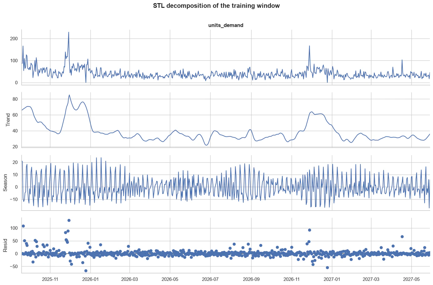
STL is a diagnostic, not a forecasting model. In this plot it provides four useful clues:
- The trend changes substantially after launch and around holiday periods, so a fixed historical mean is inadequate.
- A repeating seven-day component supports for both Holt–Winters and SARIMA.
- Seasonal amplitude varies, making multiplicative seasonality worth considering in theory, but zero-demand days make it invalid here.
- Large remainders coincide with events that trend and weekday effects cannot explain. A history-only model will continue to miss some of them.
Standard STL, Holt–Winters, and SARIMA each handle one seasonal period cleanly. If both weekly and annual seasonalities needed explicit representation, we would need an extension such as MSTL, TBATS, or dynamic harmonic regression.
ADF — Augmented Dickey–Fuller test
ADF helps assess whether ordinary differencing may be necessary. It tests whether a series contains a unit root, a common form of non-stationarity.
A weakly stationary series has an approximately constant mean, constant variance, and an autocovariance that depends on lag rather than calendar time. ARIMA needs this behaviour in the series it actually models.
The Augmented Dickey–Fuller test uses:
- : the series has a unit root and is non-stationary;
- : the series does not have a unit root under the test specification.
A common rule is:
The results are:
| Transformation | ADF statistic | p-value |
|---|---|---|
| Raw demand | −3.4328 | 0.0099 |
| First difference | −8.8361 | |
| Seasonal difference at lag 7 | −6.1794 |
Because the raw-demand p-value is below 0.05, we reject the unit-root null. That supports including candidates with : ordinary first differencing is not automatically required.
It does not prove that the raw series has no trend, seasonality, changing variance, or structural breaks. ADF addresses a specific unit-root question. Weekly differencing is still reasonable because the weekly pattern and correlation plots show a strong lag-seven relationship. We therefore test seasonal orders with both and .
ACF (Autocorrelation Function) and PACF (Partial Autocorrelation Function)
ACF identifies persistent temporal relationships, seasonal cycles, and possible moving-average structure.
The autocorrelation function measures the correlation between the series and its previous values:
at each lag . The partial autocorrelation at lag measures the incremental relationship after controlling for shorter lags.
For example:
- lag 1 compares today with yesterday;
- lag 7 compares today with the same weekday last week;
- lag 14 compares today with the same weekday two weeks ago.
Typical interpretations include:
- slow decay across many lags: differencing may be needed;
- spikes at 7, 14, and 21: weekly seasonality;
- a sharp cutoff after lag : possible MA order .
The PACF measures the direct relationship between and after controlling for the shorter lags. For example, PACF at lag 7 asks:
Does demand from seven days ago add information after accounting for lags 1 through 6?
Typical interpretations include:
- a strong lag-1 PACF: consider ;
- strong lags 1 and 2: consider ;
- a seasonal spike at lag 7: consider a seasonal AR term .
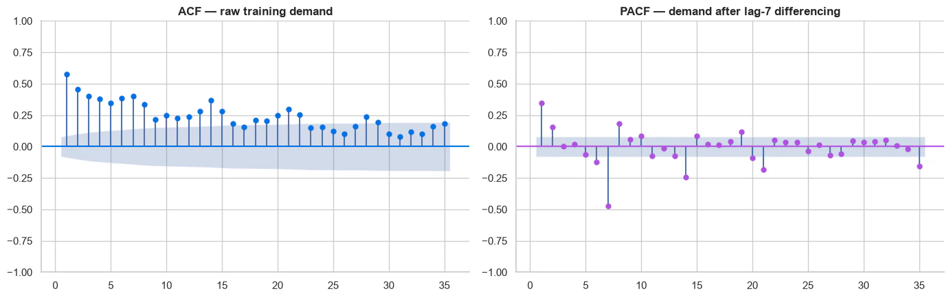
The raw ACF is strongly positive at short lags and shows recurring strength at weekly multiples. The PACF after lag-seven differencing retains a clear lag-one relationship and a smaller set of notable seasonal-multiple spikes. Together, these patterns motivate:
- a weekly period ;
- non-seasonal AR orders and as compact alternatives;
- a non-seasonal MA term ;
- testing either a seasonal AR term or a seasonally differenced MA structure with , .
ACF and PACF heuristics are cleanest for pure AR or pure MA processes. Real series with mixed AR, MA, seasonal terms, shocks, and finite samples rarely produce textbook cutoffs. They suggest a candidate set; they do not read the final orders directly from the chart.
AIC (Akaike Information Criterion) and BIC (Bayesian Information Criterion)
AIC and BIC compare fitted candidate specifications while penalising unnecessary complexity.
AIC compares statistical models by balancing likelihood fit with model complexity:
where is the likelihood and is the number of estimated parameters.
BIC uses a stronger complexity penalty:
where is the number of observations.
AIC places relatively more emphasis on predictive fit, whereas BIC's stronger penalty generally favours simpler models. Both are in-sample specification diagnostics; neither directly measures operational forecast error.
The tools play complementary roles:
| Tool | Main question | Most relevant decision |
|---|---|---|
| STL | What trend and seasonality are visible? | Seasonal period and model structure |
| ADF | Is there evidence of a unit root? | Ordinary differencing |
| ACF | Which lag correlations remain? | Seasonality, , and possible |
| PACF | Which lags have direct effects? | and possible |
| AIC/BIC | Does improved fit justify extra complexity? | Compare fitted candidates |
| Backtesting | Which candidate forecasts unseen data best? | Final model selection |
The resulting candidate set is deliberately small:
| Candidate | Validation WAPE | AIC | BIC |
|---|---|---|---|
| 27.59% | 5460.48 | 5482.92 | |
| 28.39% | 5605.04 | 5627.54 | |
| 29.35% | 5595.34 | 5622.33 | |
| 30.10% | 5612.00 | 5634.50 |
Lower is preferred among models fitted to the same target, observations, transformation, and comparable likelihood. They are valuable specification diagnostics, but they do not directly measure one-day-ahead operational error. Because differencing can also change the effective likelihood comparison, the chronological validation WAPE remains the primary selection criterion.
Evaluation metrics and model selection
No single metric describes every kind of forecast failure.
MAE: the typical miss in business units
MAE answers the most tangible question: by how many phones is the forecast wrong on an average day? Every unit of error receives equal weight.
RMSE: emphasise large misses
Squaring errors makes RMSE more sensitive to occasional large misses. This is useful when any large forecast miss is disproportionately costly. RMSE penalises overforecasting and underforecasting symmetrically; bias is still needed to describe direction. Comparing RMSE with MAE also reveals whether errors are fairly consistent or dominated by spikes.
WAPE: error relative to total demand
WAPE is the primary selection metric because it is scale-normalised, aggregates naturally across the evaluation window, and remains defined when individual days have zero demand. MAPE would divide by each actual value and therefore break on closure days.
A WAPE of 25% means total absolute error equals roughly 25% of total observed demand. It does not mean the model is “75% accurate.” Whether 25% is useful depends on the cost and tolerance of the inventory process and on performance relative to credible baselines.
Bias: the direction of total error
Negative bias means systematic underforecasting; positive bias means overforecasting. Bias cannot stand alone because positive and negative errors can cancel. A nearly unbiased model may still be highly inaccurate.
Validation selects the family winners
On the validation window, additive-trend Holt–Winters wins its family with 28.51% WAPE. The selected SARIMA specification wins its family with 27.59%. Those choices are then locked before the test window is opened.
Three simple baselines provide context. Historical mean predicts the expanding average of all demand observed so far, naive repeats yesterday's demand, and seasonal naive repeats demand from seven days earlier.
The final test results are:
| Model | MAE | RMSE | WAPE | Bias |
|---|---|---|---|---|
| Holt–Winters: additive trend + weekly | 8.87 | 11.04 | 24.43% | −0.12% |
| 8.97 | 11.16 | 24.71% | −4.45% | |
| Historical mean | 10.51 | 13.33 | 28.95% | 9.15% |
| Naive | 12.62 | 16.27 | 34.76% | 0.54% |
| Seasonal naive | 13.05 | 16.35 | 35.94% | 2.02% |
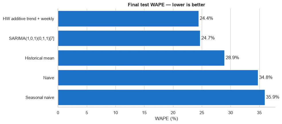
Holt–Winters lowers WAPE by about 32% relative to seasonal naive and misses by about 8.9 units on an average day. Its aggregate bias is almost zero. SARIMA is only 0.28 WAPE points behind, so the result does not justify a general claim that Holt–Winters is the superior family. It wins this particular test window.
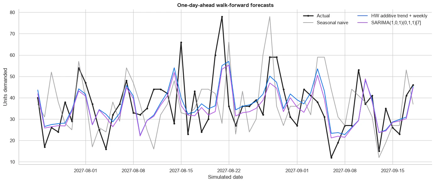
The forecast paths also show why the statistical models win: they adapt more smoothly than seasonal naive while retaining the weekly movement. None of them anticipates every sharp commercial shock.
Residual diagnostics add an important qualification. The Ljung–Box test asks whether a group of residual autocorrelations is jointly different from zero. At lags 7, 14, and 21, Holt–Winters has p-values near 0.005, evidence that temporal structure remains in its residuals. SARIMA's p-values range from 0.31 to 0.89, providing no strong evidence of remaining autocorrelation at those lags.
SARIMA is statistically cleaner; Holt–Winters is marginally more accurate on the test window. These findings are compatible. Ljung–Box asks whether residual dependence remains. WAPE asks how large the point errors were. Operational accuracy and statistical adequacy are related, but they are not the same criterion.
From point forecast to a 95% prediction interval
After evaluation, both selected models are refitted using all 730 observations. Their one-day-ahead forecasts for the next simulated date, 19 September 2027, are:
| Model | Point forecast | Lower 95% | Upper 95% |
|---|---|---|---|
| Seasonal naive | 41.0 | — | — |
| Holt–Winters | 40.0 | 10.1 | 69.8 |
| SARIMA | 39.7 | 10.9 | 68.6 |
The point forecasts are nearly identical. The test result makes Holt–Winters' 40 units the statistical recommendation, but the interval is just as important as the centre.
SARIMA's state-space likelihood produces a forecast distribution and a model-based interval. Conceptually,
with , subject to the model's residual assumptions. The Holt–Winters implementation used in the notebook does not expose an analytic interval, so its interval is an explicit Gaussian residual approximation:
Lower bounds are clipped at zero because negative unit demand is not operationally meaningful.
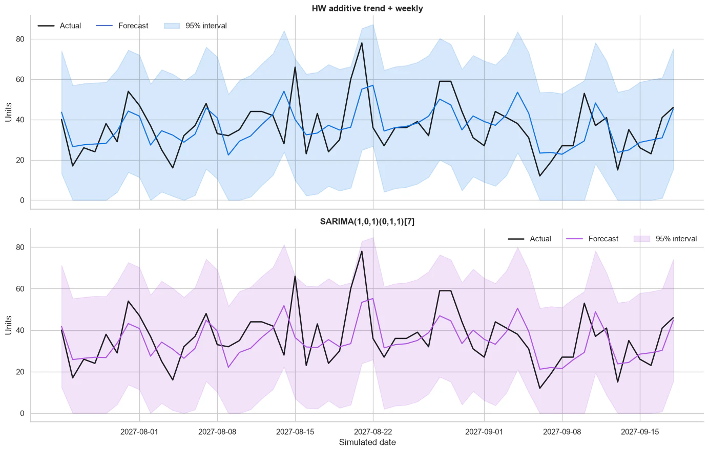
Across the 56 test days, the approximate Holt–Winters interval covers 100% of actuals with a mean width of 59.2 units. SARIMA covers 98.2% with a mean width of 57.7 units. Both coverage rates exceed the nominal 95%, suggesting that the intervals may be conservative. With only 56 observations—and an approximate Holt–Winters interval—this remains a diagnostic rather than proof of calibration.
The bands are also wide relative to mean daily demand of 39.5 units. That is an honest result. A history-only model can estimate the recurring centre of demand, but it cannot know tomorrow's promotion, competitor launch, weather, or other external shock.
These intervals quantify uncertainty; they do not prescribe an inventory target. The final step is to combine the forecast with the current inventory position, replenishment lead time, and the business cost of shortages and surplus stock.
Recommendation for inventory decision
For the next simulated day, use Holt–Winters' 40-unit forecast as the expected-demand baseline—not as the order quantity. Holt–Winters becomes the initial production model, while SARIMA continues running in parallel as a challenger.
The replenishment decision should account for the inventory already available, deliveries confirmed to arrive in time, and any safety buffer required by the chosen service level:
If expected demand is 40 units, the store has 27 units available, five more will arrive before the next selling day, and no safety buffer has yet been added, then:
The immediate replenishment requirement is eight units. This calculation assumes that replenishment can arrive before tomorrow's demand occurs. If the lead time is longer, the inventory target must cover forecast demand across the full lead-time period.
The upper end of the 95% prediction interval—approximately 70 units—should not automatically become the stock target. It describes forecast uncertainty, not the service level the business should choose. The safety buffer should instead reflect the cost of a stockout relative to the cost of carrying surplus stock.
Known promotions, launches, closures, and price changes should be recorded as explicit business adjustments because neither statistical model sees these events in advance. In production, compare Holt–Winters and SARIMA using rolling WAPE and bias alongside stockouts and excess inventory. Promote SARIMA only if it delivers a sustained improvement across these operational measures.
這篇文章是 預測 iPhone 17 Pro 需求:從統計方法到深度學習 的統計方法延伸。前文比較三類預測模型;本文則聚焦於一個更明確的問題:
僅憑歷史需求,可以把明日需求預測到多準?
這項結果會建立一個基準,後續更複雜的模型必須證明自己能穩定超越它。
本文架構如下:
1. 預測背後的決策
在虛構的倫敦市中心 Apple Store 情境中,庫存團隊每天晚上都必須決定:淺色款 iPhone 17 Pro 256GB 隔天應該準備多少台。
預測太低,門市就有缺貨、流失銷售與顧客失望的風險。預測太高,昂貴的裝置就會佔用營運資金與倉儲空間。在單一門市,這個差異或許看起來不大;但放到許多門市與眾多配置加總起來,每天微小的誤差,就會累積成一項實質的庫存決策。
因此,建模的目標是:
而營運面的問題則是:
在明天開始之前,應該備多少台?
需求預測本身不會直接決定備貨量,還需要比較缺貨成本與過剩庫存成本。若缺貨代價較高,規劃者會選擇預測分布中較高的分位數;若持有過剩庫存的代價較高,則會選擇較低的分位數。 報童模型(newsvendor model)將這個選擇表達為:
其中, 是缺貨成本, 是超額庫存成本, 代表預測需求分布的分位數函數, 則是建議庫存量。由於本實驗沒有這些成本資料,無法計算最適分位數。因此,本文只回報點預測與 95% 預測區間,服務水準仍需由業務端根據成本取捨決定。
2. 一條序列,多種行為
這個合成資料集包含 730 筆模擬的每日觀測值,時間範圍從 2025 年 9 月 19 日到 2027 年 9 月 18 日。平均每日需求為 39.5 台。模型只接收這個門市-商品組合的日期與歷史需求台數。
灰色為每日觀測值;七天移動平均線則呈現需求較緩慢的變動趨勢。
這張圖包含幾種不同型態的時間結構:
- 生命週期: 需求在上市後偏高,隨後逐漸下降到較成熟的水準。
- 每週季節性: 星期幾會改變預期需求。
- 日曆效應: 聖誕節會造成明顯的局部高峰,而公休日則可能產生真正的零需求。
- 水準變化: 兩年間,局部基準線會上升與下降,而非維持恆定。
- 不規則衝擊: 促銷與其他商業活動,會產生無法單靠趨勢或星期幾解釋的尖峰。
這是一個單變量預測問題:模型唯一可用的資訊是 的歷史紀錄。價格、促銷、行銷、假期、天氣與競爭對手動態都被刻意排除,其影響只會以模型無法直接解釋的需求衝擊反映在序列中。
這個限制其實很有用。在給機器學習模型更多特徵之前,我們想先知道:光靠需求序列本身,能解釋到什麼程度。
3. 滾動起點回測
隨機切分訓練/測試集,會讓未來的市場狀況洩漏到過去。因此,這裡改以時間順序切分觀測值:
| 區間 | 觀測值數量 | 日期 | 用途 |
|---|---|---|---|
| 訓練集 | 618 | 2025/09/19–2027/05/29 | 配適候選模型 |
| 驗證集 | 56 | 2027/05/30–2027/07/24 | 為每個模型家族選出一種規格 |
| 測試集 | 56 | 2027/07/25–2027/09/18 | 僅估計一次最終表現 |
接著,這個評估流程重現了每晚實際的作業方式:
- 使用截至第 天結束時,所有可取得的觀測值來配適模型。
- 預測第 天的需求。
- 揭曉第 天的實際需求。
- 把這筆觀測值加進可用的歷史資料中。
- 往前推進一天,重複上述步驟。
這個做法有幾種常見的稱呼:前向滾動驗證(walk-forward validation)、滾動起點評估(rolling-origin evaluation),或時間序列回測(time-series backtesting)。預測期間始終維持一天,但預測起點會隨著驗證集與測試集不斷往前推進。
每一步都只使用當時已取得的觀測值。候選規格先在驗證區間選定,再於測試區間開始前鎖定,避免測試資料影響模型設計,使評估更接近實際部署情境。
4. 傳統統計時間序列預測
Holt-Winters 與 ARIMA 都假設,序列自身的歷史紀錄包含了關於未來的有用資訊。兩者的差異,在於它們認為這些資訊該長成什麼樣子。
Holt-Winters:預測不斷演變的成分
Holt-Winters 屬於指數平滑家族。它用一組可解釋的狀態來表示時間序列:
對於季節週期為 的加法模型,狀態更新方式為:
而往前 步的預測則為:
每個狀態,都有對應的商業意涵:
- 水準 : 去除季節效應後,目前的基準值。
- 趨勢 : 這個基準值每日估計的變化量。
- 季節狀態 : 週期中某個位置的重複性效應;當 時,模型維持的是星期幾的模式。
假設現在是星期四晚上,模型要預測兩天後、星期六的需求。目前的估計值為:
- 基準需求:35 台;
- 趨勢:每天 −0.2 台;
- 星期六的季節效應:+8 台。
預測值為:
因此,模型預測大約為 43 台。
當星期六的實際需求揭曉後,Holt-Winters 會更新這三個估計值。水準參數 決定基準值反應的強度, 控制趨勢變化的速度,而 則決定這個差異中,有多少比例會被當作星期六效應本身的改變。
平滑參數 、 與 都介於 0 到 1 之間。數值愈高,對新觀測值的反應愈強烈;數值愈低,就愈能保留先前的狀態。換句話說,近期的觀測值最重要,但較舊的觀測值是逐漸淡出,而不是在某個固定的截斷點就直接消失。
當觀測值等間距、季節週期已知且穩定、水準與趨勢緩慢變化,而且異常事件不是主要訊號時,Holt-Winters 通常較為合適。加法季節性假設星期幾效應的絕對幅度大致固定;本文未採用乘法季節性,因為序列包含零需求日期,而所使用的實作要求觀測值嚴格為正。
我們驗證三種每週加法候選模型:
- 水準加季節性;
- 水準、加法趨勢與季節性;
- 水準、阻尼趨勢與季節性。
成分規格是在驗證區間中選定的;在每一種規格內,平滑係數則是從訓練歷史資料以數值方式估計出來,而非人工選定。
| Holt–Winters 候選模型 | 驗證集 MAE | 驗證集 WAPE | 偏差 |
|---|---|---|---|
| 加法趨勢 + 每週季節性 | 9.34 | 28.51% | −2.07% |
| 水準 + 每週季節性 | 9.36 | 28.57% | −1.16% |
| 阻尼趨勢 + 每週季節性 | 9.40 | 28.67% | −1.18% |
三個候選模型表現接近;加法趨勢模型的驗證集 WAPE 最低,因此被選為此模型家族的最終規格。
阻尼趨勢,會把無限外推的 項,換成一個增量效應會隨預測期間衰減的趨勢。這通常能避免不合理的長期外推,不過對於僅一天的預測而言,影響相對較小。
ARIMA:對變化、持續性與意外事件建模
Holt-Winters 透過水準、趨勢與季節性來描述需求。ARIMA 則用不同的方式處理同一個問題,它問的是:
在把序列變得足夠穩定之後,目前的需求,如何取決於過去的數值與過去的預測誤差?
這個流程可以理解為:
原始需求
      ↓ 差分
近似平穩序列
      ↓ AR 與 MA 建模
預測時間相依性
      ↓ 還原差分
還原為原始單位的需求預測
ARIMA 是 自迴歸整合移動平均模型(AutoRegressive Integrated Moving Average) 的縮寫。其表示法為 ,每個參數各自代表不同來源的資訊。
整合(I):對變化量建模,而非對水準本身建模
當 ARIMA 所建模的序列近似平穩時,通常表現最好。其平均數、變異數與相依結構,不應該隨時間出現顯著變化。
如果需求的水準或趨勢會改變,我們可以取一階差分:
此時 ARIMA 建模的不是需求本身,而是每日的變化量。假設需求從星期一的 40 台,增加到星期二的 44 台:
轉換後的觀測值就是增加了 4 台。如果套用一次一般差分,則 ;如果原始序列本身已經夠平穩,則 。
差分並不代表最終的預測結果只會以「變化量」呈現。在預測出 之後,ARIMA 會把預測出的變化量,加回最近一次觀測到的需求值上。舉例來說:
最近一次需求:             44 台
預測的每日變化量:         +3 台
預測需求:                 47 台
這個還原的動作,讓預測值回到我們真正關心的商業量值:需求台數。
自迴歸(AR):使用過去的數值
自迴歸成分假設,平穩序列或差分後序列的近期數值,可能包含關於下一個數值的資訊。
一個 AR(1) 關係式為:
其中, 是前一期的轉換後數值, 衡量它延續下去的強度, 是常數項,而 則是全新、無法預測的衝擊。
假設昨天的需求增加了 5 台,而模型估計 。那麼自迴歸成分對今天預期變化量的貢獻為:
這代表模型認為,昨天變動的一部分,很可能會延續到今天。階數 控制納入多少個過去的數值: 使用前一期的數值, 則使用前兩期的數值。
移動平均(MA):使用過去的預測誤差
移動平均成分使用的是近期的預測誤差:
前一期的誤差為:
假設昨天的預測是 40 台,但實際需求是 45 台:
模型低估了 5 台的需求。如果近期的意外落差,往往會把資訊帶到隔天,MA 成分就會利用這個誤差的一部分,來調整下一次的預測。
階數 決定使用多少個過去的誤差。儘管名稱如此,這並不是對過去需求做一般的移動平均,而是對過去預測誤差做加權組合。
結合各個成分
一個 ARIMA 模型,會先計算每日差分 ,接著使用前一期的數值與前一期的預測誤差,對這個差分建模:
最後,它會還原差分,產生以需求台數表示的預測值。用白話來說,這個模型問的是:
根據需求最近一次的變化,以及前一次預測錯了多少,我們應該預期接下來會有什麼樣的變化?
以下的一般 ARIMA 方程式,把同樣的概念延伸到任意階數 與 :
其中, 是套用 次差分之後的序列。第一個加總項,結合了前 期的轉換後數值;第二個加總項,則結合了前 期的預測誤差。本文採用 statsmodels 使用的正號慣例;部分教科書會以相反的正負號定義 MA 係數。
SARIMA:把同樣的概念延伸到每週需求
ARIMA 對近期數值與預測誤差之間的短期關係建模。SARIMA 則將這個概念延伸到重複出現的季節模式:
小寫參數描述一般的 ARIMA 行為;大寫參數則描述季節性行為:
- :季節性自迴歸階數;
- :季節性差分階數;
- :季節性移動平均階數;
- :一個季節週期中的觀測值數量。
對於具有每週模式的每日需求而言,。
季節性差分
每週的季節性差分,會將需求與一週前同一個星期幾的需求相比:
假設這個星期一的需求是 48 台,而上個星期一是 42 台:
季節性單純法(seasonal naive)假設這個差值會是零:
SARIMA 則會預測每週的變化量,並把它加到上週的需求上:
簡單來說:
季節性單純法只是重複上週的數值。SARIMA 則是從上週的數值出發,再根據近期的變化與預測誤差進行調整。
選定的模型規格
以星期一的預測為例,模型會從上個星期一的需求出發,估計需求相對於上週的變化,並根據近期的預測誤差進行調整,最後把預測出的變化量,加回上個星期一的需求上。
接下來描述的驗證流程,選出的是:
- :使用轉換後序列前一期的數值;
- :不做一般的每日差分;
- :使用一個近期的預測誤差;
- :不含季節性自迴歸項;
- :套用每週的季節性差分;
- :使用七天前的預測誤差;
- :使用七天的季節週期。
5. 我們如何選擇參數?
STL、ADF、ACF、PACF、AIC 與 BIC,能幫助我們找出合理的統計模型規格。它們各自回答不同的問題,並縮小候選集合的範圍,但並不會自動選出最終的模型——真正做出這個決定的,是依時間順序的驗證表現,以及殘差診斷。
STL——使用 LOESS 的季節趨勢分解
STL 用來探索時間序列中是否存在趨勢、季節性、季節強度的變化,或異常事件。LOESS 指的是局部估計散佈圖平滑法(Locally Estimated Scatterplot Smoothing)。使用 LOESS 的季節趨勢分解,會把訓練序列寫成
其中, 是平滑的趨勢, 是重複出現的季節成分, 則是餘量。
STL 是一種診斷工具,而不是預測模型。在這張圖中,它提供了四項有用的線索:
- 趨勢在上市之後與假期前後出現顯著變化,代表固定的歷史平均並不夠用。
- 重複出現的七天成分,支持 Holt-Winters 與 SARIMA 都採用 。
- 季節振幅會變動,理論上值得考慮乘法季節性,但由於存在零需求的日子,這裡並不適用。
- 較大的餘量,往往與趨勢和星期幾效應都無法解釋的事件同時出現。純粹只靠歷史資料的模型,仍然會持續漏掉其中一部分。
標準 STL、Holt-Winters 與 SARIMA 主要處理單一季節週期。若需要同時表示每週與年度季節性,可以考慮 MSTL、TBATS 或動態調和迴歸(dynamic harmonic regression)等延伸方法。
ADF——增強戴基-富勒檢定
ADF 能幫助我們評估是否需要進行一般差分。它檢定的是序列中是否存在單位根——這是一種常見的非平穩型態。
一個弱平穩序列,具有大致固定的平均數、固定的變異數,而自我共變異數只取決於落後期數,而不取決於實際的日曆時間。ARIMA 實際建模的序列,需要具備這樣的性質。
增強戴基-富勒檢定使用:
- (虛無假設):序列存在單位根,屬於非平穩序列;
- (對立假設):在此檢定設定下,序列不存在單位根。
常見的判斷規則是:
結果如下:
| 轉換方式 | ADF 統計量 | p 值 |
|---|---|---|
| 原始需求 | −3.4328 | 0.0099 |
| 一階差分 | −8.8361 | |
| 落後 7 期的季節性差分 | −6.1794 |
由於原始需求的 p 值低於 0.05,我們拒絕單位根的虛無假設。這支持納入 的候選模型:並不是一定需要做一般的一階差分。
但這並不能證明原始序列沒有趨勢、季節性、變異數變化,或結構性斷點。ADF 處理的,是一個特定的單位根問題。每週差分仍然是合理的選擇,因為每週模式與相關圖都顯示出強烈的落後 7 期關係。因此,我們會同時測試 與 的季節性階數。
ACF(自相關函數)與 PACF(偏自相關函數)
ACF 用來找出持續性的時間關係、季節週期,以及可能的移動平均結構。
自相關函數衡量的是,序列與其過去數值之間的相關性:
在每一個落後期 上計算。而落後期 的偏自相關,衡量的則是在控制較短落後期之後,額外增加的關係強度。
舉例來說:
- 落後 1 期,比較的是今天與昨天;
- 落後 7 期,比較的是今天與上週同一個星期幾;
- 落後 14 期,比較的是今天與兩週前同一個星期幾。
常見的解讀方式包括:
- 在許多落後期上緩慢衰減:可能需要進行差分;
- 在落後 7、14、21 期出現尖峰:代表每週季節性;
- 在落後期 之後出現明顯截斷:可能對應 MA 階數 。
PACF 衡量的是,在控制較短落後期之後, 與 之間的直接關係。舉例來說,落後 7 期的 PACF 問的是:
在考量過落後 1 到 6 期之後,七天前的需求,是否還能提供額外的資訊?
常見的解讀方式包括:
- 落後 1 期的 PACF 明顯偏高:可以考慮 ;
- 落後 1、2 期都偏高:可以考慮 ;
- 在落後 7 期出現季節性尖峰:可以考慮加入季節性 AR 項 。
原始的 ACF 在短落後期呈現強烈的正相關,並在每週倍數的落後期上重複出現較強的數值。經過落後 7 期差分後的 PACF,仍保留明顯的落後 1 期關係,以及一小組值得注意的季節倍數尖峰。綜合這些型態,可以得出以下方向:
- 每週週期 ;
- 非季節性 AR 階數 與 ,作為精簡的替代選項;
- 非季節性 MA 項 ;
- 測試季節性 AR 項 ,或是 、 的季節性差分 MA 結構,兩者皆可嘗試。
ACF 與 PACF 的典型判讀,在純 AR 或純 MA 過程中最清楚。實務序列通常同時包含 AR、MA、季節項、隨機衝擊與有限樣本誤差,因此未必會呈現教科書式的截斷。這些圖表適合用來縮小候選範圍,不能直接決定最終階數。
AIC(赤池資訊準則)與 BIC(貝氏資訊準則)
AIC 與 BIC 用來比較已配適的候選規格,同時對不必要的複雜度加以懲罰。
AIC 透過權衡概似配適度與模型複雜度,來比較統計模型:
其中, 是概似值, 是估計出的參數數量。
BIC 則使用更強的複雜度懲罰:
其中, 是觀測值的數量。
AIC 相對更重視預測配適度,而 BIC 較強的懲罰,則通常會偏好較簡單的模型。兩者都是樣本內的規格診斷工具,都不能直接衡量實際營運上的預測誤差。
這些工具彼此扮演互補的角色:
| 工具 | 主要問題 | 最相關的決策 |
|---|---|---|
| STL | 可以看到什麼樣的趨勢與季節性? | 季節週期與模型結構 |
| ADF | 是否有單位根的證據? | 一般差分 |
| ACF | 哪些落後期的相關性仍然存在? | 季節性、,以及可能的 |
| PACF | 哪些落後期具有直接效應? | ,以及可能的 |
| AIC/BIC | 配適度的改善,是否值得增加的複雜度? | 比較已配適的候選模型 |
| 回測 | 哪個候選模型對未見過的資料預測得最好? | 最終模型選擇 |
最終得到的候選集合刻意保持精簡:
| 候選模型 | 驗證集 WAPE | AIC | BIC |
|---|---|---|---|
| 27.59% | 5460.48 | 5482.92 | |
| 28.39% | 5605.04 | 5627.54 | |
| 29.35% | 5595.34 | 5622.33 | |
| 30.10% | 5612.00 | 5634.50 |
在目標變數、觀測值、轉換方式相同,且概似值具有可比性的模型之間,數值愈低愈好。這些指標是很有價值的規格診斷工具,但並不能直接衡量隔天預測的實際誤差。由於差分也可能改變概似值比較的有效性,依時間順序的驗證集 WAPE,仍然是主要的選擇標準。
6. 評估指標與模型選擇
沒有單一指標,能夠描述所有類型的預測失誤。
MAE:以商業單位表示的典型誤差
MAE 回答的是最直觀的問題:平均而言,每天的預測誤差是幾台手機?每一台的誤差,權重都相同。
RMSE:放大較大的誤差
將誤差平方,讓 RMSE 對偶發的大誤差更敏感。當任何一次大幅失準的預測,代價都不成比例地高時,這項指標就特別有用。RMSE 對高估與低估的懲罰是對稱的;要描述誤差的方向,仍然需要偏差指標。比較 RMSE 與 MAE,也能看出誤差是相當一致,還是主要由少數尖峰所主導。
WAPE:相對於總需求的誤差
WAPE 是主要的選擇指標,因為它經過尺度標準化、能自然地在整個評估區間中加總,而且即使個別日期需求為零,也仍然有定義。MAPE 則是除以每一天各自的實際值,因此在公休日就會失效。
WAPE 為 25%,代表總絕對誤差,大約等於總觀測需求的 25%。這並不代表模型「準確率是 75%」。25% 是否算是可用的表現,取決於庫存流程的成本與容忍度,也取決於相對於可信基準模型的表現。
偏差:總誤差的方向
負偏差代表系統性低估;正偏差代表系統性高估。偏差不能單獨使用,因為正負誤差可能會互相抵銷——一個幾乎沒有偏差的模型,仍然可能非常不準確。
以驗證集選擇各模型家族的最終規格
在驗證區間中,加法趨勢的 Holt-Winters 以 28.51% 的 WAPE,在自己的模型家族中勝出;選定的 SARIMA 規格,則以 27.59% 在其家族中勝出。這些選擇會在打開測試區間之前先行鎖定。
三個簡單的基準模型提供了對照的脈絡。歷史平均法預測的是截至目前為止所有需求的擴張平均數;**單純法(naive)**重複昨天的需求;季節性單純法則重複七天前的需求。
最終的測試結果為:
| 模型 | MAE | RMSE | WAPE | 偏差 |
|---|---|---|---|---|
| Holt–Winters:加法趨勢 + 每週季節性 | 8.87 | 11.04 | 24.43% | −0.12% |
| 8.97 | 11.16 | 24.71% | −4.45% | |
| 歷史平均法 | 10.51 | 13.33 | 28.95% | 9.15% |
| 單純法 | 12.62 | 16.27 | 34.76% | 0.54% |
| 季節性單純法 | 13.05 | 16.35 | 35.94% | 2.02% |
相較於季節性單純法,Holt-Winters 把 WAPE 降低了約 32%,平均每天的誤差約為 8.9 台,整體偏差幾乎為零。SARIMA 的 WAPE 只落後 0.28 個百分點,因此這個結果並不足以支持「Holt-Winters 是整體上更優越的模型家族」這種普遍性的說法——它只是在這個特定的測試區間中勝出。
預測路徑也顯示出,為什麼這兩個統計模型會勝出:它們的調整方式比季節性單純法更平滑,同時仍保留每週的變動。但它們都無法預先掌握每一次劇烈的商業衝擊。
殘差診斷則加上了一項重要的但書。Ljung-Box 檢定問的是,一組殘差自相關是否整體顯著不為零。在落後 7、14、21 期,Holt-Winters 的 p 值接近 0.005,顯示其殘差中仍殘留著時間結構。SARIMA 在這些落後期的 p 值介於 0.31 到 0.89 之間,並沒有強烈證據顯示仍存在自相關。
SARIMA 的殘差診斷較理想,Holt-Winters 在測試區間的點預測則略為準確。兩項結果並不矛盾:Ljung-Box 檢驗殘差是否仍存在自相關,WAPE 衡量的則是點預測誤差。統計診斷與實際預測表現彼此相關,但不是同一項標準。
7. 從點預測到 95% 預測區間
評估完成之後,兩個選定的模型都會使用全部 730 筆觀測值重新配適。它們對下一個模擬日期——2027 年 9 月 19 日——的隔日預測為:
| 模型 | 點預測 | 95% 下界 | 95% 上界 |
|---|---|---|---|
| 季節性單純法 | 41.0 | — | — |
| Holt–Winters | 40.0 | 10.1 | 69.8 |
| SARIMA | 39.7 | 10.9 | 68.6 |
兩者的點預測幾乎相同。根據測試結果,統計上建議採用 Holt-Winters 的 40 台這個數字,但預測區間本身,和中心點同樣重要。
SARIMA 的狀態空間概似函數,會產生一個預測分布,以及以模型為基礎的預測區間。概念上為:
其中 ,並受限於模型對殘差的假設。筆記本中使用的 Holt-Winters 實作,並未提供解析形式的預測區間,因此這裡改用明確的高斯殘差近似:
下界會被截斷在零,因為負的需求台數在營運上沒有意義。
在 56 天的測試期間中,Holt-Winters 的近似區間涵蓋了 100% 的實際值,平均寬度為 59.2 台;SARIMA 則涵蓋了 98.2%,平均寬度為 57.7 台。兩者的涵蓋率,都超過名目上的 95%,顯示這些區間可能偏保守。由於樣本只有 56 筆——且 Holt-Winters 的區間本身就是近似值——這仍然只能算是一項診斷,而不是校準良好的證明。
相較於每日平均需求 39.5 台,這些區間相當寬。這反映出單變量模型的限制:它能估計需求的重複性結構,卻無法預先得知促銷、競品上市、天氣變化或其他外部衝擊。
這些區間量化的是不確定性,並不能直接指定庫存目標。最後一步,是把預測結果,與目前的庫存部位、補貨前置時間,以及缺貨與庫存過剩的商業成本結合起來考量。
8. 庫存決策建議
對於下一個模擬日期,應該把 Holt-Winters 預測出的 40 台,當作預期需求的基準值——而不是直接當作訂購數量。Holt-Winters 會成為初始的正式模型,而 SARIMA 則會以挑戰模型的角色,持續並行運作。
補貨決策,應該將目前已有的庫存、已確認能及時送達的貨量,以及所選服務水準所需的任何安全緩衝,都納入考量:
如果預期需求為 40 台,門市目前有 27 台庫存,另外還有 5 台會在下一個銷售日之前送達,且尚未加入任何安全緩衝,那麼:
立即需要補貨的數量就是 8 台。這個計算假設補貨能在明天需求發生之前送達;如果前置時間更長,庫存目標就必須涵蓋整個前置時間期間的預測需求。
95% 預測區間的上界——大約 70 台——不應該自動被當作庫存目標。它描述的是預測的不確定性,而不是企業應該選擇的服務水準。安全緩衝,應該反映的是缺貨成本相對於持有過剩庫存成本的高低。
已知的促銷、新品上市、公休與價格變動,都應該記錄為明確的業務調整項目,因為這兩個統計模型都無法預先看到這些事件。在正式上線後,應該用滾動的 WAPE 與偏差,搭配缺貨與庫存過剩的實際情況,來比較 Holt-Winters 與 SARIMA。只有當 SARIMA 在這些營運指標上,展現出持續性的改善時,才應該將它升級為正式模型。