How We Got to LLMs: From Word2Vec to the Transformer大型語言模型如何演進:從 Word2Vec 到 Transformer
Four architectural leaps—word embeddings, RNNs, the Transformer, and scale—each one a fix for the last one's limit, and the reason today's LLMs are capable, confident, and occasionally wrong.從詞嵌入、RNN 到 Transformer 與規模化,四次關鍵的技術躍進如何突破前一階段的限制,並塑造今日 LLM 的能力與局限。
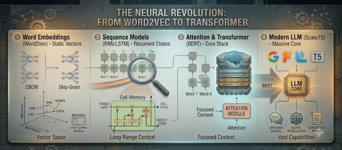
When ChatGPT appeared, it felt as though AI had suddenly learned to speak. It can feel like a new kind of technology, but LLMs are not new — and they did not begin with ChatGPT. There is no official point at which a language model becomes a large language model. No governing body sets a minimum parameter count, and no single paper marks its birth. If we need a starting point for the modern LLM, 2017 is the clearest answer. That was the year researchers introduced the Transformer — the architecture behind nearly every major LLM today.
BERT and GPT followed, demonstrating what happened when Transformers were pretrained on large amounts of text. GPT-2 was already being described as a “large language model” in 2019; GPT-3 then showed how dramatically new capabilities could emerge as models grew. ChatGPT brought those capabilities to the public—it did not create them (Transformer paper, 2019 usage of “large language model”, GPT-3 paper).
Transformer did not appear from nowhere. It was the result of a chain of breakthroughs stretching back years: word embeddings gave words mathematical meaning, recurrent networks introduced memory, attention helped models focus, and Transformers made the whole process scalable. So the story of LLMs does not begin with a chatbot—or even with something we would call an LLM today. It begins with a more fundamental problem:
How can a machine represent and understand language at all?
This article explores that question in two parts. First, The evolution of language models offers a conceptual walkthrough of four major eras—what each introduced, where it fell short, and how those limitations led to the next breakthrough. Then, Text summarization using four eras of models turns theory into a practical comparison: we give each generation the same summarization task and compare how the models—and their results—have changed.
The evolution of language models
Stage 1: Word Embeddings — Words Become Numbers (2013)
Before 2013, a word was just an index in a lookup table. "Car" and "automobile" were as unrelated to a model as "car" and "trombone"—two arbitrary IDs, no matter how close their meaning.
Word embedding (e.g., Word2Vec) changed the representation. The core idea is that similar things should be close together in vector space; dissimilar things should be far apart. Instead of an ID, embeddings turn every word into a dense vector representation that captures its semantic meaning. We can think of an embedding as a list of a few hundred numbers—learned by analyzing the contexts in which a word appears.
For the first time, "meaning" was something you could measure with a distance function. Distance in that vector space started to encode similarity in meaning: "king" lands much closer to "queen" than to "banana," because king and queen keep turning up in similar contexts and banana never does. The famous example:
Nobody told the model that "king" and "queen" differ by gender the same way "man" and "woman" do. It fell out of the geometry, purely from co-occurrence statistics.
Details of Word2Vec
The core idea of Word2Vec is to learn word representations by predicting context from words (or vice versa). Based on the distributional hypothesis — "a word is characterized by the company it keeps."
- Two Architectures
Word2Vec comes in two mirror-image flavors. Skip-gram—the more common of the two—takes a center word and predicts the words around it: "given 'cat,' predict 'the,' 'sat,' 'on,' 'mat.'" CBOW does the reverse: given the surrounding words, predict the one in the middle.
| Architecture | Task | Intuition |
|---|---|---|
| Skip-gram | Predict context words given center word | "Given 'cat', predict 'the', 'sat', 'on','mat'" |
| CBOW (Continuous Bag of Words) | Predict center word given context | "Given 'the', 'sat', 'on', 'mat', predict 'cat'" |
Walking through skip-gram: for every word in the corpus, take a window of words on either side, and treat each (center, context) pair as one training example.
The model itself is simple — one-hot encode the center word, multiply by an embedding matrix W to select its vector, multiply that by a second matrix W'
to get a score for every word in the vocabulary, then softmax to turn scores into probabilities. Train it so the true context words score high.
Input: center word (one-hot, dim V)
         ↓
       [W: V×D]             ← input embedding matrix — this is what we keep!
         ↓
   hidden layer (dim D)     ← this word's embedding vector (typically 100-300)
         ↓
       [W′: D×V]            ← output embedding (context) matrix — typically discarded
         ↓
  softmax over vocabulary
         ↓
 predicted context word
 (repeated once per position in the window)
- Negative Sampling
One practical problem: that softmax sums over the entire vocabulary on every single training example—potentially hundreds of thousands of words. The trick that makes this computationally viable is negative sampling. Instead of scoring every word in the vocabulary, the model compares the true context word against a handful of random "noise" words (typically 5–20), and is trained to prefer the real pair over the fakes.
The objective function for a single target word and a single context word is to maximize the following expression:
Where:
- is the sigmoid function
- First term: Pushes the positive pair closer together, maximizing the probability of the positive sample. For the pair , should be close to 1.
- Second term: Pushes the negative pairs apart, minimizing the probability of the negative samples. For the noise pair , should be close to 0.
- is the number of negative samples (a hyperparameter, usually 5 to 20).
- is the noise distribution used for sampling negative words. The 0.75 exponent smooths the distribution—giving rare words a slightly higher chance of being sampled as negatives.
That turns an expensive vocabulary-wide classification problem (softmax) into a handful of cheap yes/no (sigmoid) questions per example. This optimization is largely why the model was trainable at scale in 2013.
The embedding you actually keep afterward — the one behind "king − man + woman ≈ queen" — is just W, the input matrix. W' gets thrown away once training finishes.
The Wall: The classical word embedding (e.g. Word2Vec) gives every word exactly one vector. "Bank" gets a single point in space, shared between "river bank" and "bank account" — the word means two different things, but the model only has one representation for it. Also, Word2Vec has no opinion on how to combine word vectors into a sentence; it understands words, not order.
Stage 2: Sequence Models — Language Gains Memory (2014–2016)
If word order matters — and "dog bites man" means something very different from "man bites dog" — a model needs to process words in sequence, not as a bag of vectors.
Recurrent Neural Networks (RNNs) do exactly that. They process a sequence by reading one token, updating an internal hidden state (memory), reading the next token, and updating again.
        x_1         x_2         x_3
         ↓           ↓           ↓
... → [RNN]   →  [RNN]   →  [RNN] → ...
       (h_1)       (h_2)       (h_3)
Because the representation of a word now depends on the hidden state accumulated from the words before it, context emerges. "Bank" after "river" and "bank" after "savings" can now result in different final representations, because the model has actually processed what preceded each one.
While elegant, vanilla RNNs suffer from a fatal flaw: it is not capable of handling a long text and it quickly "forgets" distant words. This make it unable to learn long-range dependencies.
Details of Vanilla RNN
At each time step , a basic RNN takes the current input vector (the word embedding) and the previous hidden state to compute the new hidden state:
While elegant, vanilla RNNs suffer from a fatal flaw: the vanishing gradient problem. During backpropagation through time (BPTT), gradients are repeatedly multiplied by the weight matrix . If these weights are small, the gradients shrink exponentially toward zero as they move backward through the sequence. The model quickly "forgets" distant words, making it unable to learn long-range dependencies.
Long Short-Term Memory (LSTM) refine this with gates that explicitly decide what to keep, update, or discard from memory — a more disciplined version of the same idea.
Details of LSTM
LSTM networks refine this by introducing a secondary memory stream called the cell state () and using learnable gates to explicitly decide what information to keep, update, or discard. Inside an LSTM cell, four distinct neural network layers work in tandem:
- Forget Gate: Decides what to discard from the past memory.
- Input Gate & Candidate Cell: The input gate () decides what new information to store, while a layer creates a vector of new candidate values ().
- Cell State Update: The old memory is multiplied by the forget gate (fading irrelevant past context), and the new candidate values are scaled by the input gate and added. This creates a constant gradient path through time, bypassing the vanishing gradient problem.
- Output Gate: Decides what part of the internal cell state makes it to the visible hidden state for the next step in the sequence.
The wall: information has to travel through the sequence one step at a time. By the time a long sentence's tenth word arrives, whatever mattered from the first word has usually faded — long-range relationships are hard to preserve, even with an LSTM's gating. And because each step depends on the one before it, an RNN can't be unrolled and processed all at once: training time scales with sequence length and can't be efficiently parallelized across a GPU.
Stage 3: Attention and the Transformer — Every Token Can Look at Every Other Token (2017–2018)
Attention lets a model connect relevant words directly, no matter how far apart they sit in a sentence. A preliminary version of this idea was patched into RNNs back in 2014, allowing a decoder to look back across everything an encoder had seen instead of relying on a single compressed summary vector.
In 2017, a paper with a blunt title took that patch and made it the entire architecture. "Attention Is All You Need" processes every token in parallel, using attention alone to relate tokens to each other—no recurrence required.
RNN: A time-dependent chain
[Token 1] ──> [Token 2] ──> [Token 3] ──> [Token 4]
   ↓             ↓             ↓             ↓
(step 1)      (step 2)      (step 3)      (step 4)


Transformer: A parallel grid
[Token 1]     [Token 2]     [Token 3]     [Token 4]
   │             │             │             │
   └─────────────┴──────┬──────┴─────────────┘
                        ↓ (Self-Attention)
   ┌─────────────┬──────┴──────┬─────────────┐
   ↓             ↓             ↓             ↓
(step 1)      (step 1)      (step 1)      (step 1)
Under the hood, "related to each other" is driven by a specific mechanism worth naming. Every token produces three learned vectors:
- a Query — what it is looking for,
- a Key — what it has to offer, and
- a Value — what it actually contributes.
Each token's query is compared against every other token's key. Those comparison scores are turned into weights, and the token's new representation becomes a weighted blend of every other token's value.
Details of Attention
The Attention mechanism is fundamentally a differentiable dictionary lookup, computed as a series of matrix multiplications.
1. Creating the Matrices:
For a sequence of tokens represented by a matrix , the model learns three distinct weight matrices (). Multiplying the input by these weights creates the Query, Key, and Value matrices:
2. The Score (Dot Product):
By taking the dot product of the Queries and the Keys, the model calculates an matrix (where is the sequence length). This matrix represents the raw affinity score between every single word and every other word in the sequence.
3. Scaling:
If the dimensionality of the keys () is large, the dot products can grow massively, pushing the softmax function into regions where gradients approach zero. Dividing by stabilizes the variance and ensures smooth training.
4. The Weights:
Applying the softmax function normalizes the scores along each row so they sum to 1. This creates a grid of attention weights, telling each token exactly how much "attention" to pay to every other token.
5. The Output:
Finally, multiplying this weight matrix by the Value matrix () produces the new token representations. If the word "bank" pays 90% of its attention to "river" and 10% to "mud," its new vector will be a 90/10 weighted average of their respective Value vectors.
(Note: The full Transformer actually uses Multi-Head Attention, running this exact formula multiple times in parallel with different weight matrices to capture different linguistic relationships simultaneously — e.g., one head might look for subjects/verbs, while another looks for adjectives).
The part worth sitting with: every token can pull from every other token in the sequence, all at once. It doesn't just look at the one word directly before it, and it isn't limited by whatever an RNN's memory managed to carry forward.
The headline benefit isn't just accuracy, though—it is economics. Every position in the sequence can now be computed simultaneously. Matrix multiplications are exactly what GPUs are designed to do. That is what made training on internet-scale text affordable. The Transformer's real contribution was making scale possible, not making language understanding "solved."
A quick correction: The original 2017 Transformer is not encoder-only, and it isn't decoder-only either. It is an encoder-decoder, built specifically for machine translation. An encoder reads the source sentence; a decoder generates the target sentence, attending back to the encoder as it goes. What came next was researchers taking different halves of that same architecture to build the models we use today:
- Encoder-decoder — the original design. The encoder builds a rich representation of the input; the decoder generates an output while attending to it. This remains the natural fit for tasks with a clear input-to-output shape, like translation (e.g., T5, BART).
- Encoder-only — BERT (2018). Keeps just the encoder half, reading a sequence in both directions at once. It is pretrained by masking random words and predicting them, then fine-tuned per task. Built for understanding text rather than generating it, it dominated NLP benchmarks for two years and, within 18 months, was powering a large share of Google Search.
- Decoder-only — GPT (2018 onward). Keeps just the decoder half, reading strictly left-to-right to predict the next token. Built to generate, not just represent.
The wall: BERT's paradigm requires a labeled dataset and a fresh fine-tuning run for every new task—one model for sentiment analysis, another for entity extraction, another for Q&A. The decoder-only line pointed toward something more general (prompting a single model to do anything), but GPT-1 and GPT-2 were not yet robust enough to prove the idea had no ceiling. Going into 2020, that was still an open question.
(BERT's lineage didn't die, by the way — it lives on as the embedding models behind modern semantic search.)
Stage 4: The Modern LLM Recipe — Decoder-Only Transformers and the Scale Era (2020–Present)
While the public timeline of generative AI seems to start in late 2022, the actual architectural turning point happened in 2020. That was the year the decoder-only architecture won the argument that GPT-1 and GPT-2 couldn't settle—and it won it purely on scale, in a way nobody had fully predicted.
In May 2020, GPT-3 was released at 175 billion parameters (roughly 500x the size of BERT-Large). At that size, it could perform tasks it was never explicitly trained on, specified entirely through a few examples in the prompt. Nobody engineered that behavior in; it emerged. Parameter counts jumped, capability jumped with them in ways that weren't linearly predictable, and "large" stopped being just a decorative adjective. The field started saying LLM.
The result of this pure scaling was a base model with genuine capability but terrible manners—it could generate incredibly realistic text, but it had no real sense of being asked a question. It was a massive autocomplete engine. It took two years of engineering to solve that final piece. Instruction tuning and alignment (using Reinforcement Learning from Human Feedback) closed the gap, transforming the raw GPT-3 architecture into the highly aligned ChatGPT in late 2022.
Strip away the magic, and what was left circa 2020 was a relatively simple recipe—dense, decoder-only Transformers trained on raw internet scrapes. As dense scaling hit hardware and data limits, that recipe had to evolve. Today's state-of-the-art looks vastly different:
- From Dense to Sparse (MoE): We no longer activate every parameter for every word. Trillion-parameter models now use a Mixture of Experts, dynamically routing each token to specialized sub-networks to massively increase capacity without exploding inference costs.
- The Data Wall and Synthetic Data: We have largely exhausted the high-quality public internet. Frontier models are now trained on highly curated synthetic data—often generated and verified by other models—prioritizing dense reasoning, math, and code over raw web scrapes.
- Inference-Time Compute: Autoregressive prediction is no longer just a fast reflex. The modern edge involves training models to "think" (plan, search, and self-correct via hidden reasoning tokens) during inference, trading immediate response time for much deeper logical accuracy.
- Agentic Workflows and Tool Use: We have moved beyond passive chatbots. The LLM is now the central reasoning engine for autonomous agents that can plan multi-step workflows, write and execute their own code, query live databases, call external APIs, and interact with the physical and digital world.
- Native Multimodality: We stopped bolting vision and audio tools onto text models. Modern architectures tokenize text, audio, and video directly into the same latent space from day one.
We have moved from static lookup tables to dynamic sequences, to parallel attention grids, and finally to trillion-parameter reasoning engines. The cleanest way to see exactly how far we have come across this entire evolution is to put one model from every era above through the exact same task.
Text summarization task using four eras of models
The history becomes more concrete when every era faces the same job. For this comparison, I created 2,400 fictional product reviews, each paired with a one-sentence reference summary. The first 2,000 reviews form the training split, 200 are reserved for validation, and 200 form the test split. Every system below was evaluated on the same first 20 held-out test reviews.
This is deliberately a small architectural demonstration, not a leaderboard. The systems differ in size, pretraining, supervision, and whether they extract or generate text. The dataset is also template-generated rather than written by real customers. Those differences make the historical progression visible, but they prevent a clean claim that architecture alone caused any score change.
Here is the first test review:
The WorkNest Chair has been part of my routine for six weeks. It looked much like the photos and felt familiar within a day. Assembly is straightforward with clear instructions. The chair creaks and feels less sturdy than expected. The seat cushion flattens too quickly. The adjustment range is too limited. The drawbacks outweigh the few things it does well.
The reference summary is:
The WorkNest Chair has decent assembly, but weak comfort makes it difficult to recommend.
The task sounds simple: compress seven sentences into one short verdict. But doing that well requires several separate abilities—identifying important sentences, preserving sentiment, combining evidence, and writing something that is both concise and faithful.
1. Word2Vec: represent, average, and copy
Word2Vec is not a summarizer by itself. In this experiment, it provides the representation inside a classical extractive pipeline.
I trained 100-dimensional skip-gram embeddings on the 2,000 training reviews.
word2vec = Word2Vec(
    sentences=corpus,  # Tokenized documents. Each element should look like ["battery", "life", "is", "good"]
    vector_size=100,   # Number of values in each word embedding. Larger vectors can capture more relationships but require more data, memory, and computation.
    window=5,          # Maximum context distance around the target word.
    min_count=3,       # Minimum total frequency required for a word to enter the vocabulary.
    workers=max(1, (os.cpu_count() or 2) - 1),
    sg=1,              # 1. skip-gram, 0 CBOW
    negative=10,       # Number of negative examples
    epochs=6,
    seed=SEED,
)
Each sentence becomes the average of its word vectors; averaging all sentence vectors produces a document centroid. The pipeline ranks sentences by cosine similarity to that centroid, adds a small position bonus, and copies at most two high-ranking sentences in their original order.
def summarize_word2vec(document, word_budget=WORD_BUDGET):
    # 1. Break the review document into sentences.
    sentences = split_sentences(document)
    if not sentences:
        return ""

    # 2. Represent every sentence as one vector.
    vectors = [sentence_vector(sentence) for sentence in sentences]

    # 3. Average all sentence vectors to represent the whole document.
    centroid = np.mean(vectors, axis=0)

    # 4. Score sentences by similarity to the document, with a small preference for earlier sentences.
    bias = 0.08
    scores = [cosine(vector, centroid) + bias / (index + 1) for index, vector in enumerate(vectors)]

    # 5. Select the highest-scoring sentences.
    chosen, words = [], 0
    for index in np.argsort(scores)[::-1]:
        sentence_words = len(tokenize(sentences[index]))

        # Skip a sentence if it would exceed the desired length.
        if chosen and words + sentence_words > word_budget:
            continue
        chosen.append(int(index))
        words += sentence_words

        # Stop after reaching the budget or selecting two sentences.
        if words >= word_budget or len(chosen) == 2:
            break

    # 6. Restore the sentences to their original document order.
    return " ".join(sentences[index] for index in sorted(chosen))
For the WorkNest review, it returns:
It looked much like the photos and felt familiar within a day. The adjustment range is too limited.
The second sentence is useful, but the first is generic setup rather than the review's verdict. More importantly, the two claims remain disconnected. The pipeline cannot rewrite them as “limited adjustability makes the chair difficult to recommend,” because its output vocabulary consists of complete source sentences.
This is the consequence of both the representation and the decision rule. Averaging word vectors discards order, gives every occurrence of a word the same meaning, and reduces a sentence to one point. Centroid similarity then asks which sentence is most typical of the document—not necessarily which one a reader most needs to know.
Across the 20 reviews, this system achieved a ROUGE-L score of 0.174 and a source four-gram copy rate of 0.916. It was effectively instantaneous at 0.00038 seconds per review on the test machine. That combination—fast, faithful to the source wording, but shallow—is exactly what we should expect from static embeddings plus sentence ranking.
2. A hierarchical BiLSTM: learn which sentences matter
The second system replaces averaged static vectors with a recurrent model. A word-level bidirectional LSTM reads each sentence; a sentence-level bidirectional LSTM then reads the sequence of sentence representations. The result is an importance score for every sentence in the review.
class HierarchicalBiLSTM(nn.Module):
    def __init__(self, vocab_size, embedding_dim=96, hidden_dim=48):
        super().__init__()

        # Word embedding layer: (batch, sentences, words, embed_size)
        self.embedding = nn.Embedding(vocab_size, embedding_dim, padding_idx=0)

        # Word-level BiLSTM, this LSTM reads the words inside each sentence.
        # forward state:  48 values + backward state: 48 values => return 96 values (hidden_dim * 2)
        self.word_lstm = nn.LSTM(embedding_dim, hidden_dim, batch_first=True, bidirectional=True)

        # Sentence-level BiLSTM, the second BiLSTM reads the sentence representations in document order:
        self.sentence_lstm = nn.LSTM(hidden_dim * 2, hidden_dim, batch_first=True, bidirectional=True)
        self.dropout = nn.Dropout(0.2) # Dropout is disabled during evaluation after.

        # Sentence classifier converts its 96-dimensional contextual representation into one number.
        self.classifier = nn.Linear(hidden_dim * 2, 1)

    def forward(self, documents):
        """
        documents: 3-D tensor. (batch_size, max_sentences, max_words)
        """
        batch, sentence_count, word_count = documents.shape

        # Flatten documents into sentences. (16, 30, 36) -> (480, 36)
        flat = documents.reshape(batch * sentence_count, word_count)

        # Embed words and run the word-level LSTM: (480, 36)-> (480, 36, 96)
        word_states, hidden_cell = self.word_lstm(self.embedding(flat))

        # Identify real words. unsqueeze(-1) adds a feature dimension so the mask can be applied across all 96 hidden features.
        word_mask = flat.ne(0).unsqueeze(-1) # (480, 36) → (480, 36, 1)

        # Why fill padding with -1e4? If padding were filled with zero, it might incorrectly win when all real activations for a feature are negative:
        sentence_vectors = word_states.masked_fill(~word_mask, -1e4).max(dim=1).values
        has_words = flat.ne(0).any(dim=1, keepdim=True)
        sentence_vectors = torch.where(has_words, sentence_vectors, torch.zeros_like(sentence_vectors))

        # Reconstruct the document hierarchy: (480, 96) -> (16, 30, 96)
        sentence_vectors = sentence_vectors.reshape(batch, sentence_count, -1)

        # Run the sentence-level BiLSTM
        document_states, _ = self.sentence_lstm(sentence_vectors)

        # Apply dropout and classification: (16, 30, 96)-> (16, 30, 1) -> (16, 30)
        return self.classifier(self.dropout(document_states)).squeeze(-1)
The training data contains reference summaries but no human labels saying which source sentences are important. To create supervision, each training sentence is compared with its review's reference using ROUGE-L. The best-matching sentence becomes a positive ROUGE-derived pseudo-label. At test time, the model sees only the review and predicts sentence importance on its own.
Its summary for the same review is:
The WorkNest Chair has been part of my routine for six weeks. The adjustment range is too limited.
This is still extractive, so it cannot synthesize a new sentence. But it now preserves the product name and selects a concrete weakness. Across the test set, ROUGE-L rises to 0.220, the best result among the three systems before the instruction-tuned LLM.
The improvement comes with two qualifications. First, the model learns the biases of its pseudo-labeling rule: “best lexical match to the reference” is not identical to “most important sentence.” Second, the output still copies the source. Its four-gram copy rate remains 0.836. Recurrence improves the representation of order and context, but it does not by itself make a system abstractive; the output objective still asks this model to select sentences.
The recurrent architecture also retains the limitation described in part one. Word states must be computed in sequence, and information reaches distant positions through repeated updates. The hierarchy shortens that path by modeling words within sentences and then sentences within documents, but it does not remove the sequential bottleneck.
3. An encoder–decoder Transformer: attention plus generation
The first two systems use extractive summarization: they select and copy sentences from the source. Stage 3 moves to abstractive summarization, which generates a new summary and can paraphrase or combine information.
This stage uses DistilBART-CNN, an encoder–decoder Transformer fine-tuned for news summarization. The encoder reads the full review, while the decoder uses cross-attention to consult the source as it generates each output token.
from transformers import AutoModelForSeq2SeqLM, AutoTokenizer
MODEL_NAME = 'sshleifer/distilbart-cnn-12-6'
tokenizer = AutoTokenizer.from_pretrained(MODEL_NAME)
model = AutoModelForSeq2SeqLM.from_pretrained(MODEL_NAME).to(device).eval()

...

def summarize_transformer(document):
    inputs = tokenizer(
        document,
        return_tensors='pt', # returns PyTorch tensors.
        truncation=True,
        max_length=MAX_INPUT_TOKENS
    ).to(device)
    with torch.inference_mode(): # Disable training-related calculations
        generated = model.generate(
            **inputs, num_beams=4, do_sample=False, min_new_tokens=12, max_new_tokens=80,
            length_penalty=1.0, no_repeat_ngram_size=3, early_stopping=True,
        )
    return tokenizer.decode(generated[0], skip_special_tokens=True).strip()
For the WorkNest review, it produces:
Assembly is straightforward with clear instructions. The drawbacks outweigh the few things it does well. The chair creaks and feels less sturdy than expected.
Although DistilBART is an abstractive summarizer capable of generating new wording, it mostly copies and reorders the source sentences. Its 0.803 four-gram copy rate confirms this behavior across the test set.
Its ROUGE-L score is 0.172, slightly below Word2Vec and the BiLSTM. DistilBART also produces the longest summaries, adding words that do not overlap with the concise references and lowering its ROUGE score.
What the stage does demonstrate cleanly is the removal of the fixed recurrent bottleneck. The encoder maintains a contextual representation for every source position, and each generated token can retrieve different evidence through cross-attention. The model no longer has to compress the entire review into one final recurrent state before it begins writing.
4. An instruction-tuned decoder-only LLM: the task moves into the prompt
The final system is Qwen2.5-1.5B-Instruct, a 1.54-billion-parameter decoder-only Transformer.
from transformers import AutoModelForCausalLM, AutoTokenizer

MODEL_NAME = 'Qwen/Qwen2.5-1.5B-Instruct'
tokenizer = AutoTokenizer.from_pretrained(MODEL_NAME)
model = AutoModelForCausalLM.from_pretrained(MODEL_NAME, torch_dtype=dtype).to(device).eval()

...

def summarize_llm(document):
    messages = [
        {'role': 'system', 'content': SYSTEM_PROMPT},
        {'role': 'user', 'content': 'Summarize this user review:\n\n' + document},
    ]
    input_ids = tokenizer.apply_chat_template(
        messages,
        tokenize=True,
        add_generation_prompt=True,
        return_tensors='pt',
        truncation=True,
        max_length=MAX_INPUT_TOKENS,
    ).to(device)
    with torch.inference_mode():
        generated = model.generate(
            input_ids,
            max_new_tokens=80,
            do_sample=False,
            repetition_penalty=1.05,
            pad_token_id=tokenizer.eos_token_id,
        )
    new_tokens = generated[0, input_ids.shape[-1]:]
    summary = tokenizer.decode(new_tokens, skip_special_tokens=True).strip()
    return summary.removeprefix('Summary:').strip()
It receives no summarization training in this experiment. Instead, its chat prompt specifies the task:
You summarize product reviews. Return exactly one concise factual sentence that captures
the overall sentiment and the most important strength or weakness. Use only the review.
It returns:
The WorkNest Chair, while familiar and easy to assemble, falls short in comfort and adjustability, with issues like frequent creaking, rapid seat cushion flattening, and limited adjustment range, which outweigh its initial positive impression.
This is the first output that behaves like an editor rather than a sentence selector. It names the product, preserves the negative verdict, and combines several pieces of evidence into a grammatical sentence. Across all 20 reviews, it achieved the highest ROUGE-L score, 0.266, while its four-gram copy rate fell to 0.031. In other words, only about 3% of its four-word sequences were copied directly from the source.
The flexibility is not free. Average inference time rose to 0.570 seconds per review, excluding model loading. More importantly, generation introduces a failure mode that strict extraction cannot have: a fluent model can change a fact.
Two test outputs show the risk. One source says the DustPilot 3 “maps rooms and moves around furniture reliably”; Qwen summarizes that it “doesn't map rooms as accurately as some other models.” Another says the MetroPods connection “stays stable”; the generated summary introduces “occasional stability issues.” Both sentences sound plausible, and both reverse or invent evidence. The instruction “use only the review” reduces this risk but does not eliminate it.
Reading the results without turning them into a leaderboard
| System | How it summarizes | ROUGE-L | Compression ratio | Source 4-gram copy rate | Seconds per review |
|---|---|---|---|---|---|
| Word2Vec + centroid ranking | Selects source sentences with static embeddings | 0.174 | 0.367 | 0.916 | 0.00038 |
| Hierarchical BiLSTM | Learns to select source sentences | 0.220 | 0.336 | 0.836 | 0.006 |
| DistilBART-CNN | Generates with an encoder–decoder Transformer | 0.172 | 0.463 | 0.803 | 0.378 |
| Qwen2.5-1.5B-Instruct | Generates from a natural-language instruction | 0.266 | 0.397 | 0.031 | 0.570 |
ROUGE-L measures overlap with a reference, not truth. Compression ratio measures length, not completeness. Copy rate measures reuse, not quality. Latency depends on hardware and decoding settings. The table is useful only when read together with the actual outputs.
Three patterns are more informative than the ranking:
- Representation and output strategy are separate choices. The BiLSTM understands order but remains extractive because it was trained to score sentences. DistilBART can generate new wording but often copies because that is what its learned distribution favors.
- Attention changes how evidence is available. The Transformer encoder keeps a contextual state for every source token, and cross-attention lets the decoder retrieve from those states while writing. This is the structural break from recurrence.
- Instruction tuning changes the interface. In the first three systems, summarization behavior is encoded in ranking logic, pseudo-labels, or task-specific fine-tuning. In the fourth, a substantial part of the specification is expressed in ordinary language. The prompt becomes part of the program.
The progression is therefore not simply “each model scores higher.” It is a shift in where the capability lives. Word2Vec supplies reusable word geometry to an algorithm. The BiLSTM learns contextual sentence importance. The encoder–decoder Transformer learns to read and write with direct access to the source. The instruction-tuned LLM turns summarization into one behavior of a general model—more flexible and more fluent, but also more capable of being confidently wrong.
當 ChatGPT 問世時,許多人彷彿第一次看見 AI 真正「學會說話」。然而,大型語言模型(LLM)並非憑空出現,它的技術源流也遠早於 ChatGPT。
語言模型究竟從何時起才算是「大型」,學界並沒有正式分界。目前既沒有統一的參數量門檻,也沒有單一篇論文可以被視為 LLM 的明確起點。
如果要為現代 LLM 選擇一個具代表性的起點,2017 年是合理的答案。那一年,研究者提出 Transformer,奠定了今日多數主流 LLM 的架構基礎。
隨後問世的 BERT 與 GPT,進一步展示了在大量文本上預訓練 Transformer 所能帶來的能力。早在 2019 年,GPT-2 就已被稱為「大型語言模型」;GPT-3 則進一步顯示,模型規模擴大後,能展現出新的任務能力。ChatGPT 的重要性,在於將這些能力帶入大眾使用情境,而非從零創造它們(參見 Transformer 論文、2019 年「大型語言模型」一詞的使用,以及 GPT-3 論文)。
Transformer 並非憑空出現。它是一連串技術突破累積多年的成果:詞嵌入賦予文字數學上的意義,循環神經網路引入了記憶能力,注意力機制讓模型懂得聚焦重點,而 Transformer 則讓整個過程得以規模化。因此,LLM 的故事並不是從聊天機器人開始的——甚至不是從今天我們會稱之為 LLM 的東西開始的。它始於一個更根本的問題:
機器究竟要如何表徵並理解語言?
本文分為兩部分。第一部分〔語言模型的演進〕從概念上梳理四個主要階段:每個階段解決了什麼問題、遇到哪些瓶頸,以及這些限制如何推動下一次技術突破。第二部分〔以四個世代的模型做文本摘要任務〕則將概念落實為實驗:讓四個世代的模型處理同一項摘要任務,比較模型架構與輸出如何演變。
語言模型的演進
第一階段:詞嵌入——將文字轉換為向量(2013)
在 2013 年之前,一個詞對模型來說就只是查找表裡的一個索引。「car」和「automobile」在模型眼中,跟「car」和「trombone」一樣毫無關聯——無論語意多麼接近,它們都只是兩個任意的編號。
詞嵌入(例如 Word2Vec)改變了這種表示方式。其核心概念是:意義相近的事物,在向量空間中應該彼此靠近;意義不同的事物則應該相距較遠。嵌入不再用單一編號代表一個詞,而是將每個詞轉換成一個能捕捉其語意的稠密向量。我們可以把嵌入想像成一串數百個數字——這串數字是透過分析該詞出現的上下文學習而來的。
從此,語意相似度首次可以透過向量距離加以量化。在向量空間中,「king」會靠近「queen」,卻遠離「banana」,因為 king 與 queen 經常出現在相似的語境中,而 banana 的使用情境明顯不同。
最著名的例子:
沒有人告訴模型「king」與「queen」之間的性別差異,和「man」與「woman」之間的性別差異是同一種關係。這個結果純粹是從共現統計中,自然而然從向量的幾何結構中浮現出來的。
Word2Vec 的技術細節
Word2Vec 的核心概念,是透過「用詞預測上下文」(或反過來)來學習詞的表示方式。這個想法奠基於分佈假說——「一個詞的意義,取決於與它相伴出現的詞」。
- 兩種架構
Word2Vec 有兩種互為鏡像的版本。Skip-gram——兩者中較常見的一種——會拿一個中心詞,去預測它周圍的詞:「給定『cat』,預測『the』、『sat』、『on』、『mat』」。CBOW 則反過來:給定周圍的詞,去預測中間那個詞。
| 架構 | 任務 | 直觀理解 |
|---|---|---|
| Skip-gram | 給定中心詞,預測上下文詞 | 「給定『cat』,預測『the』、『sat』、『on』、『mat』」 |
| CBOW(連續詞袋模型) | 給定上下文詞,預測中心詞 | 「給定『the』、『sat』、『on』、『mat』,預測『cat』」 |
以 skip-gram 為例來說明:對語料庫中的每一個詞,取其左右兩側一定範圍內的詞,並將每一組(中心詞,上下文詞)視為一筆訓練樣本。
模型本身相當單純——將中心詞做 one-hot 編碼,乘上嵌入矩陣 W 以選出對應的向量,再乘上第二個矩陣 W',
得到詞彙表中每個詞的分數,最後用 softmax 把分數轉換成機率。訓練的目標,就是讓真正的上下文詞獲得高分。
輸入:中心詞(one-hot 編碼,維度 V)
         ↓
       [W: V×D]             ← 輸入嵌入矩陣 —— 這是我們最後保留下來的東西!
         ↓
   隱藏層(維度 D)          ← 這個詞的嵌入向量(通常為 100–300 維)
         ↓
       [W′: D×V]            ← 輸出(上下文)嵌入矩陣 —— 通常訓練後會捨棄
         ↓
     對整個詞彙表做 softmax
         ↓
      預測出的上下文詞
   (視窗中每個位置各重複一次)
- 負採樣(Negative Sampling)
這裡有個實際的問題:每一筆訓練樣本,這個 softmax 都得對整個詞彙表求和——而詞彙表可能有數十萬個詞。讓這件事在計算上可行的關鍵技巧,就是負採樣。與其為詞彙表中每個詞都打分數,模型改成只拿真正的上下文詞,去和少數幾個(通常 5 到 20 個)隨機抽出的「雜訊」詞做比較,並訓練模型偏好真實配對、而非假的配對。
對於單一目標詞 與單一上下文詞 ,其目標函數是要最大化以下這個式子:
其中:
- 是 sigmoid 函數
- 第一項:讓正樣本配對更靠近彼此,最大化正樣本的機率。對配對 而言, 應該要接近 1。
- 第二項:讓負樣本配對彼此遠離,最小化負樣本的機率。對雜訊配對 而言, 應該要接近 0。
- 是負樣本的數量(一個超參數,通常介於 5 到 20 之間)。
- 是用來抽取負樣本詞的雜訊分布。指數 0.75 的作用是讓分布變得平滑——讓罕見詞被抽中作為負樣本的機率略微提高。
這麼一來,原本昂貴、需要對整個詞彙表分類的問題(softmax),就被轉化成每筆樣本只需回答少數幾個廉價的是非題(sigmoid)。這項優化,正是 2013 年這個模型得以大規模訓練的主要原因。
訓練結束後真正保留下來的嵌入向量——也就是「king − man + woman ≈ queen」背後的那組向量——其實就是輸入矩陣 W。訓練一結束,W' 就會被捨棄。
極限所在: 傳統詞嵌入(例如 Word2Vec)為每個詞只提供唯一一個向量。「bank」在空間中只對應到一個點,「river bank」(河岸)和「bank account」(銀行帳戶)共用這同一個點——這個詞明明有兩種截然不同的意思,模型卻只有一種表示方式。此外,Word2Vec 對於該如何將這些詞向量組合成一個句子,完全沒有想法;它理解的是詞,而不是詞序。
第二階段:序列模型——語言擁有了記憶(2014–2016)
如果詞序真的重要——而「dog bites man」(狗咬人)和「man bites dog」(人咬狗)的意思顯然天差地遠——那麼模型就必須按順序處理詞語,而不是把它們當成一袋雜亂的向量。
循環神經網路(RNN) 正是為此而生。它逐一讀入 token,更新內部的隱藏狀態(也就是記憶),再讀入下一個 token,再次更新——如此反覆進行。
        x_1         x_2         x_3
         ↓           ↓           ↓
... → [RNN]   →  [RNN]   →  [RNN] → ...
       (h_1)       (h_2)       (h_3)
由於一個詞的表示方式,現在取決於它前面所有詞累積下來的隱藏狀態,語境於是就此浮現。出現在「river」之後的「bank」,和出現在「savings」之後的「bank」,如今可以得到不同的最終表示,因為模型確實「讀過」各自前面出現了什麼。
這個設計雖然優雅,但最原始的 RNN 卻有一個致命缺陷:它無法妥善處理較長的文本,而且很快就會「遺忘」較遠處的詞。這使得它難以學會長距離的依賴關係。
原始 RNN 的技術細節
在每個時間步 ,基本的 RNN 會取用當前的輸入向量 (也就是詞嵌入)與前一步的隱藏狀態 ,計算出新的隱藏狀態:
這個設計雖然優雅,卻有一個致命缺陷:梯度消失問題。在「隨時間反向傳播」(BPTT)的過程中,梯度會被反覆乘上權重矩陣 。如果這些權重數值偏小,梯度在沿著序列反向傳遞時,就會呈指數級縮小、趨近於零。於是模型很快就會「遺忘」較遠處的詞,也就難以學會長距離的依賴關係。
長短期記憶網路(LSTM) 進一步改良了這個想法,加入了「閘門」機制,明確決定要保留、更新或捨棄記憶中的哪些內容——可以說是同一套想法更有紀律的版本。
LSTM 的技術細節
LSTM 網路的改良方式,是額外引入一條稱為「細胞狀態」()的記憶流,並透過可學習的閘門,明確決定要保留、更新或捨棄哪些資訊。 在一個 LSTM 單元內部,有四個不同的神經網路層協同運作:
- 遺忘閘(Forget Gate):決定要從過去的記憶中捨棄哪些內容。
- 輸入閘與候選細胞狀態:輸入閘()決定要儲存哪些新資訊,而一層 則會產生一組候選值向量()。
- 細胞狀態更新:舊有的記憶 會先乘上遺忘閘(讓不相關的過去語境逐漸淡化),接著新的候選值會依輸入閘的比例縮放後加入。 這樣的設計,會在時間軸上創造出一條穩定的梯度傳遞路徑,藉此繞過梯度消失問題。
- 輸出閘:決定內部細胞狀態中,有哪一部分會傳遞到外顯的隱藏狀態 ,供序列中的下一步使用。
極限所在: 資訊必須沿著序列一步一步地傳遞。當一個長句傳遞到第十個詞時,第一個詞原本重要的資訊往往早已淡化——即使有 LSTM 的閘門機制,長距離的關係依然難以保留。而且,因為每一步都依賴前一步的結果,RNN 無法被展開後一次性平行處理:訓練所需的時間會隨序列長度增加,也無法在 GPU 上有效平行運算。
第三階段:注意力機制與 Transformer——讓 token 直接交換資訊(2017–2018)
注意力機制讓模型能夠直接連結彼此相關的詞,無論它們在句子中相隔多遠。這個想法的雛形,早在 2014 年 就已整合進 RNN,讓解碼器能夠回頭參照編碼器處理過的所有位置,而不再只依賴單一的壓縮向量。
到了 2017 年,〈Attention Is All You Need〉將注意力機制從 RNN 的輔助元件,提升為整個架構的核心。它讓所有 token 可以平行處理,並透過注意力機制建立位置之間的關聯,不再依賴循環結構。
RNN:依時間順序的鏈狀結構
[Token 1] ──> [Token 2] ──> [Token 3] ──> [Token 4]
   ↓             ↓             ↓             ↓
(步驟 1)      (步驟 2)      (步驟 3)      (步驟 4)


Transformer:平行的網格結構
[Token 1]     [Token 2]     [Token 3]     [Token 4]
   │             │             │             │
   └─────────────┴──────┬──────┴─────────────┘
                        ↓(自注意力)
   ┌─────────────┬──────┴──────┬─────────────┐
   ↓             ↓             ↓             ↓
(步驟 1)      (步驟 1)      (步驟 1)      (步驟 1)
在底層,「彼此相關」其實是由一個值得特別說明的具體機制所驅動。每個 token 都會產生三個學習得來的向量:Query(查詢)——代表它在尋找什麼;Key(鍵)——代表它能提供什麼;以及 Value(值)——代表它實際貢獻的內容。每個 token 的 Query 都會與其他所有 token 的 Key 相互比較,這些比較分數會被轉換成權重,而該 token 的新表示,就是其他所有 token 的 Value 依權重加權混合而成的結果。
注意力機制的技術細節
注意力機制本質上是一種可微分的字典查詢,透過一連串的矩陣乘法運算完成。
1. 建立矩陣:
對於用矩陣 表示的 token 序列,模型會學習三個不同的權重矩陣()。將輸入乘上這些權重,就能得到 Query、Key、Value 三個矩陣:
2. 分數計算(點積):
透過將 Query 與 Key 做點積,模型會算出一個 的矩陣(其中 為序列長度)。這個矩陣代表了序列中每一個詞與其他每一個詞之間的原始關聯分數。
3. 縮放:
如果 Key 的維度()很大,點積的數值可能會變得非常大,使 softmax 函數落入梯度趨近於零的區域。除以 能穩定變異數,確保訓練過程順利進行。
4. 權重計算:
套用 softmax 函數,會將每一列的分數正規化,使其總和為 1。這樣就會產生一整個注意力權重的網格,明確告訴每個 token:該對其他每一個 token 分配多少「注意力」。
5. 輸出:
最後,將這個權重矩陣乘上 Value 矩陣(),就會得到每個 token 全新的表示。如果「bank」把 90% 的注意力放在「river」上、10% 放在「mud」上,那麼它的新向量,就會是這兩者各自 Value 向量依 90/10 比例加權平均後的結果。
(補充說明:完整的 Transformer 實際上採用的是多頭注意力(Multi-Head Attention),也就是用不同的權重矩陣,將這同一套公式平行執行多次,藉此同時捕捉不同層面的語言關係 ——例如,某一個「頭」可能專門尋找主詞與動詞的關係,另一個頭則專門找形容詞。)
這項設計的關鍵在於:每個 token 都能直接從序列中允許參照的其他 token 取得資訊。它不只參照緊接在前的詞,也不再受限於 RNN 單一隱藏狀態所能保留的內容。
不過,這項設計的核心優勢不只在模型品質,更在於計算效率。序列中的各個位置可以同時運算,而矩陣乘法正是 GPU 擅長處理的工作。這使得在網路規模的文本上進行訓練成為可能。Transformer 的關鍵貢獻,是讓模型得以有效擴大規模,而不是徹底解決「語言理解」問題。
一個常見的誤解需要澄清:2017 年最原始的 Transformer,既不是純編碼器(encoder-only),也不是純解碼器(decoder-only)架構。它是一個編碼器-解碼器(encoder-decoder)架構,最初是專為機器翻譯而設計的。編碼器負責讀取來源句子;解碼器則一邊生成目標句子,一邊回頭參照編碼器的內容。後來研究者做的事,是把這同一套架構拆成不同的一半,打造出我們今天所使用的模型:
- 編碼器-解碼器(Encoder-decoder) —— 最原始的設計。編碼器負責建立輸入內容豐富的表示;解碼器則一邊參照這個表示,一邊生成輸出。對於輸入與輸出之間有明確對應關係的任務(例如翻譯),這仍然是最自然的選擇(如 T5、BART)。
- 純編碼器(Encoder-only)——BERT(2018)。 只保留編碼器這一半,能夠同時雙向讀取整個序列。它的預訓練方式,是隨機遮蔽部分詞彙並要求模型預測,之後再針對各項任務個別微調。這種架構主要用於建立文字的雙向表示,而非直接生成文字。BERT 曾長時間主導多項 NLP 評測,並快速被應用於 Google 搜尋等實際系統。
- 純解碼器(Decoder-only)——GPT(2018 年起)。 只保留解碼器這一半,嚴格依由左至右的順序讀取,並預測下一個 token。這種架構是為了「生成」而生,而不只是「表示」文字。
極限所在: BERT 這套典範,每次面對新任務都需要一份標註資料集,並重新進行一輪微調——情感分析要一個模型,實體擷取要另一個模型,問答系統又要再另一個模型。純解碼器這條路線,則指向了某種更為通用的可能性(只需對單一模型下指令,就能完成各種任務),但 GPT-1 與 GPT-2 當時的能力,還不足以證明這個想法真的沒有上限。一直到 2020 年,這仍是一個懸而未決的問題。
(順帶一提,BERT 這一脈並沒有就此消失——它以嵌入模型的形式延續至今,正是現代語意搜尋背後的重要推手。)
第四階段:現代 LLM 的配方——純解碼器 Transformer 與規模化時代(2020 年至今)
雖然在大眾的認知裡,生成式 AI 的時間軸似乎是從 2022 年底才開始,但真正的架構轉捩點其實發生在 2020 年。就是在那一年,純解碼器架構終於贏得了 GPT-1 與 GPT-2 都未能定論的那場爭辯——而且贏得的方式,純粹是靠「規模」,而這是當時沒有人完全預料到的。
2020 年 5 月,GPT-3 問世,擁有 1,750 億個參數(大約是 BERT-Large 的 500 倍)。在這樣的規模下,它能夠完成從未被明確訓練過的任務,只需在提示詞中給出幾個範例即可。這種能力並不是被特意設計出來的,而是自然湧現的。參數量跳升,能力也隨之躍升,而且這種躍升並不是線性可預測的,「大型」(large)從此不再只是個裝飾性的形容詞。整個領域,開始把這類模型稱為 LLM。
規模化帶來了能力強大、但尚未對齊使用者意圖的基礎模型。它能產生高度流暢的文字,卻未必能辨識使用者是在提問、下指令,或單純要求續寫;從功能上看,它仍是一個大規模的自動續寫模型。之後,指令微調與基於人類回饋的強化學習(RLHF)進一步縮小這項落差,讓原始的 GPT-3 架構逐步發展成 2022 年底推出的 ChatGPT。
撇開這些看似神奇的表象,2020 年前後留下來的,其實是一份相對簡單的配方——密集(dense)、純解碼器的 Transformer,訓練資料則是從網路上原始擷取的文本。然而,隨著密集規模化逐漸撞上硬體與資料的極限,這份配方也不得不跟著演變。今天最先進的做法,看起來已經截然不同:
- 從密集走向稀疏(MoE):我們不再讓每個詞都啟動全部的參數。如今擁有兆級參數的模型,會採用專家混合模型(Mixture of Experts, MoE)架構,動態地將每個 token 導向特定的專門子網路,藉此大幅提升模型容量,卻不會讓推論成本跟著暴增。
- 資料牆與合成資料:公開網路上高品質的文本,如今已幾乎被用盡。前沿模型現在大量仰賴經過精心篩選的合成資料——這些資料通常是由其他模型生成、再經其他模型驗證——比起原始網路擷取的資料,更著重密集推理、數學與程式碼能力。
- 推論時運算(Inference-Time Compute):自迴歸預測不再只是一種快速的反射動作。如今的技術前緣,在於訓練模型在推論階段「思考」(透過隱藏的推理 token 進行規劃、搜尋與自我修正),用即時反應速度換取遠遠更深的邏輯準確度。
- 代理式工作流程與工具使用:我們已經走出被動聊天機器人的階段。LLM 如今成為自主代理(agent)背後的核心推理引擎,能夠規劃多步驟的工作流程、自行撰寫並執行程式碼、查詢即時資料庫、呼叫外部 API,並與實體及數位世界互動。
- 原生多模態:我們不再只是把視覺與語音工具硬生生接到文字模型上。現代架構從一開始,就將文字、音訊、影像直接 token 化,統一映射進同一個潛在空間之中。
我們已經從靜態的查找表,走到動態的序列,再走到平行的注意力網格,最終來到兆級參數的推理引擎。要清楚看見這整段演進究竟走了多遠,最直接的方式,就是讓上述每個世代各挑一個模型,去面對完全相同的任務。
以四個世代的模型做文本摘要任務
當每個世代都面對同一份工作時,前面談到的這段歷史就會變得更加具體。為了這項比較,我建立了 2,400 篇虛構的產品評論,每篇都搭配一句參考摘要。前 2,000 篇評論作為訓練集,200 篇保留作為驗證集,另外 200 篇則作為測試集。以下每一套系統,都是在同樣的前 20 篇保留測試評論上進行評估。
這刻意設計成一個小規模的架構示範,而非一場排行榜競賽。這幾套系統在規模、預訓練方式、監督訊號,以及究竟是「擷取」還是「生成」文字上,都各有不同。此外,這份資料集也是以樣板方式產生,而非真實顧客所撰寫。這些差異讓歷史的演進脈絡得以清楚呈現,但也使我們無法乾脆地宣稱:分數上的任何變化,純粹是架構本身造成的。
以下是第一篇測試評論:
英文原文: The WorkNest Chair has been part of my routine for six weeks. It looked much like the photos and felt familiar within a day. Assembly is straightforward with clear instructions. The chair creaks and feels less sturdy than expected. The seat cushion flattens too quickly. The adjustment range is too limited. The drawbacks outweigh the few things it does well.
中文翻譯: 我已經使用 WorkNest 這張椅子六週了。它看起來和照片十分相似,用了一天就覺得很順手。組裝過程簡單,說明書也很清楚。不過,椅子會發出吱嘎聲,結構也不如預期穩固;座墊很快就塌陷,可調整範圍也太小。整體而言,缺點多於優點。
參考摘要為:
英文原文: The WorkNest Chair has decent assembly, but weak comfort makes it difficult to recommend.
中文翻譯: WorkNest 這張椅子組裝體驗尚可,但舒適度不足,使人難以推薦。
這項任務聽起來很簡單:把七個句子濃縮成一句簡短的結論。但要把這件事做好,其實需要好幾種不同的能力——判斷哪些句子重要、保留原本的情感傾向、整合各項證據,並寫出一段既精簡又忠於原文的文字。
1. Word2Vec:表示、平均、複製
Word2Vec 本身並不是一個摘要系統。在這項實驗中,它是在一套傳統的抽取式流程裡,負責提供文字的向量表示。
我在這 2,000 篇訓練評論上,訓練了 100 維的 skip-gram 嵌入向量。
word2vec = Word2Vec(
    sentences=corpus,  # 已斷詞的文件。每個元素形式類似 ["battery", "life", "is", "good"]
    vector_size=100,   # 每個詞嵌入向量的維度。維度越大能捕捉越多關係,但也需要更多資料、記憶體與運算量。
    window=5,          # 目標詞前後可考慮的最大上下文距離。
    min_count=3,       # 一個詞要進入詞彙表所需的最低總出現頻率。
    workers=max(1, (os.cpu_count() or 2) - 1),
    sg=1,              # 1 代表 skip-gram,0 代表 CBOW
    negative=10,       # 負樣本的數量
    epochs=6,
    seed=SEED,
)
每個句子的向量,是其內部所有詞向量的平均值;再將所有句子向量平均,就能得到整篇文件的中心點(centroid)。這套流程會依據與該中心點的餘弦相似度為句子排序,額外加上一個小幅度的位置加成,並依原始順序,最多複製兩個排名最高的句子。
def summarize_word2vec(document, word_budget=WORD_BUDGET):
    # 1. 將評論文件切分成句子。
    sentences = split_sentences(document)
    if not sentences:
        return ""

    # 2. 將每個句子表示成一個向量。
    vectors = [sentence_vector(sentence) for sentence in sentences]

    # 3. 將所有句子向量平均,代表整篇文件。
    centroid = np.mean(vectors, axis=0)

    # 4. 依與文件的相似度為句子打分,並給予較前面句子些微的加成。
    bias = 0.08
    scores = [cosine(vector, centroid) + bias / (index + 1) for index, vector in enumerate(vectors)]

    # 5. 選出分數最高的句子。
    chosen, words = [], 0
    for index in np.argsort(scores)[::-1]:
        sentence_words = len(tokenize(sentences[index]))

        # 若加入這句會超出預期長度,就跳過這句。
        if chosen and words + sentence_words > word_budget:
            continue
        chosen.append(int(index))
        words += sentence_words

        # 達到字數預算或已選滿兩句後就停止。
        if words >= word_budget or len(chosen) == 2:
            break

    # 6. 將選出的句子還原成原文中的順序。
    return " ".join(sentences[index] for index in sorted(chosen))
針對這篇 WorkNest 的評論,它輸出的結果是:
英文原文: It looked much like the photos and felt familiar within a day. The adjustment range is too limited.
中文翻譯: 它看起來和照片十分相似,用了一天就感覺很熟悉。可調整的範圍也太小。
第二句確實有用,但第一句只是泛泛的背景鋪陳,而不是評論真正的結論。更重要的是,這兩個論點彼此毫無連結。這套流程沒有辦法把它們改寫成「可調整性不足,使這張椅子難以推薦」這樣的句子,因為它能輸出的內容,就只能是原文中完整的句子。
這是「表示方式」與「決策規則」兩者共同造成的結果。將詞向量取平均,會捨棄詞序、讓同一個詞的每一次出現都被視為同一種意思,並把整個句子壓縮成空間中的單一一點。而中心點相似度所問的問題,是「哪個句子最能代表整篇文件」——這未必等同於「讀者最需要知道哪一句」。
在這 20 篇評論上,這套系統的 ROUGE-L 分數為 0.174,來源文字的四連詞(four-gram)複製率為 0.916。在測試機器上,處理速度幾乎是即時的,平均每篇評論僅需 0.00038 秒。這樣的組合——快速、忠於原文用字,卻流於表面——正是靜態嵌入加上句子排序這套方法所應該預期的結果。
2. 階層式 BiLSTM:學習判斷哪些句子重要
第二套系統,用循環模型取代了「取平均的靜態向量」。詞層級的雙向 LSTM 會逐句閱讀;句子層級的雙向 LSTM,則接著閱讀這些句子表示所構成的序列。最終的結果,是為評論中每一個句子都算出一個重要性分數。
class HierarchicalBiLSTM(nn.Module):
    def __init__(self, vocab_size, embedding_dim=96, hidden_dim=48):
        super().__init__()

        # 詞嵌入層:(batch, sentences, words, embed_size)
        self.embedding = nn.Embedding(vocab_size, embedding_dim, padding_idx=0)

        # 詞層級 BiLSTM,負責讀取每個句子內部的詞。
        # 正向狀態:48 維 + 反向狀態:48 維 => 共輸出 96 維(hidden_dim * 2)
        self.word_lstm = nn.LSTM(embedding_dim, hidden_dim, batch_first=True, bidirectional=True)

        # 句子層級 BiLSTM,依文件中的順序讀取各句子的表示:
        self.sentence_lstm = nn.LSTM(hidden_dim * 2, hidden_dim, batch_first=True, bidirectional=True)
        self.dropout = nn.Dropout(0.2) # 評估階段會停用 Dropout。

        # 句子分類器,將 96 維的上下文表示轉換成單一一個數值。
        self.classifier = nn.Linear(hidden_dim * 2, 1)

    def forward(self, documents):
        """
        documents:三維張量。(batch_size, max_sentences, max_words)
        """
        batch, sentence_count, word_count = documents.shape

        # 將文件攤平成句子。(16, 30, 36) -> (480, 36)
        flat = documents.reshape(batch * sentence_count, word_count)

        # 對詞做嵌入,並執行詞層級 LSTM:(480, 36)-> (480, 36, 96)
        word_states, hidden_cell = self.word_lstm(self.embedding(flat))

        # 找出真正的詞(而非填補值)。unsqueeze(-1) 新增一個特徵維度,讓遮罩能套用到全部 96 個隱藏特徵上。
        word_mask = flat.ne(0).unsqueeze(-1) # (480, 36) → (480, 36, 1)

        # 為什麼用 -1e4 來填補?如果用 0 來填補,當某個特徵的所有真實激活值都是負的時候,填補值反而可能會被誤判為最大值:
        sentence_vectors = word_states.masked_fill(~word_mask, -1e4).max(dim=1).values
        has_words = flat.ne(0).any(dim=1, keepdim=True)
        sentence_vectors = torch.where(has_words, sentence_vectors, torch.zeros_like(sentence_vectors))

        # 還原文件的階層結構:(480, 96) -> (16, 30, 96)
        sentence_vectors = sentence_vectors.reshape(batch, sentence_count, -1)

        # 執行句子層級 BiLSTM
        document_states, _ = self.sentence_lstm(sentence_vectors)

        # 套用 dropout 並分類:(16, 30, 96)-> (16, 30, 1) -> (16, 30)
        return self.classifier(self.dropout(document_states)).squeeze(-1)
訓練資料雖然附有參考摘要,卻沒有人工標註哪些原文句子才是重要的。為了建立監督訊號,每一個訓練句子都會用 ROUGE-L 與該評論的參考摘要進行比較。匹配程度最高的句子,就會被當作正向的 ROUGE 衍生偽標籤。到了測試階段,模型只會看到評論本身,並自行預測每個句子的重要程度。
它對同一篇評論產生的摘要為:
英文原文: The WorkNest Chair has been part of my routine for six weeks. The adjustment range is too limited.
中文翻譯: 我已經使用 WorkNest 這張椅子六週了。它的可調整範圍太小。
這仍然是抽取式的方法,所以無法合成出全新的句子。不過,它現在保留了產品名稱,也選出了一個具體的缺點。在整個測試集上,ROUGE-L 分數提升到 0.220,是在指令微調 LLM 之前,三套系統中表現最好的一個。
這樣的進步伴隨著兩點但書。第一,模型學到的其實是偽標籤規則本身的偏誤:「與參考摘要在字面上最匹配」並不等同於「真正最重要的句子」。第二,輸出結果依然是複製原文而來,其四連詞複製率仍高達 0.836。循環結構確實改善了對詞序與語境的表示能力,但這件事本身並不會讓一套系統變得「生成式」;這個模型的輸出目標,終究還是在「挑選句子」。
這種循環架構,也依然保留了第一部分所提到的那個限制。詞的狀態必須依序計算,資訊要傳到較遠的位置,得靠一次又一次的更新才能抵達。這種階層式設計,透過「先在句子內建模詞、再在文件內建模句子」的方式縮短了這條路徑,但並沒有真正消除序列化這個瓶頸本身。
3. 編碼器-解碼器 Transformer:注意力機制加上生成能力
前兩套系統採用的都是抽取式摘要:從原文中挑選並複製句子。第三階段則邁向生成式摘要,能夠產生全新的摘要文字,也能改寫或整合不同的資訊。
這個階段使用的是 DistilBART-CNN,一個針對新聞摘要微調過的編碼器-解碼器 Transformer。編碼器負責讀取整篇評論,解碼器則在生成每一個輸出 token 時,透過交叉注意力機制回頭參照原文。
from transformers import AutoModelForSeq2SeqLM, AutoTokenizer
MODEL_NAME = 'sshleifer/distilbart-cnn-12-6'
tokenizer = AutoTokenizer.from_pretrained(MODEL_NAME)
model = AutoModelForSeq2SeqLM.from_pretrained(MODEL_NAME).to(device).eval()

...

def summarize_transformer(document):
    inputs = tokenizer(
        document,
        return_tensors='pt', # 回傳 PyTorch 張量。
        truncation=True,
        max_length=MAX_INPUT_TOKENS
    ).to(device)
    with torch.inference_mode(): # 停用與訓練相關的計算
        generated = model.generate(
            **inputs, num_beams=4, do_sample=False, min_new_tokens=12, max_new_tokens=80,
            length_penalty=1.0, no_repeat_ngram_size=3, early_stopping=True,
        )
    return tokenizer.decode(generated[0], skip_special_tokens=True).strip()
針對這篇 WorkNest 的評論,它產生的結果是:
英文原文: Assembly is straightforward with clear instructions. The drawbacks outweigh the few things it does well. The chair creaks and feels less sturdy than expected.
中文翻譯: 組裝過程簡單,說明書也很清楚。整體而言,缺點蓋過了它少數做得不錯的地方。椅子會發出吱嘎聲,坐起來也不如預期那麼穩固。
雖然 DistilBART 是一套能夠生成全新文字的生成式摘要系統,但它多半只是複製並重新排列原文的句子。整個測試集上 0.803 的四連詞複製率,也證實了這種行為模式。
它的 ROUGE-L 分數為 0.172,略低於 Word2Vec 與 BiLSTM。DistilBART 也產生了最長的摘要,其中加入了不少與簡潔的參考摘要並不重疊的字詞,因而拉低了它的 ROUGE 分數。
不過,這個階段確實清楚展示了一件事:固定的循環瓶頸已被移除。編碼器為原文中的每一個位置,都維持著各自的上下文表示,而每一個生成出來的 token,都能透過交叉注意力取用不同的證據。模型不必再像過去那樣,得先把整篇評論壓縮進一個最終的循環狀態,才能開始下筆。
4. 指令微調的純解碼器 LLM:任務被搬進了提示詞裡
最後一套系統是 Qwen2.5-1.5B-Instruct,一個擁有 15.4 億參數的純解碼器 Transformer。
from transformers import AutoModelForCausalLM, AutoTokenizer

MODEL_NAME = 'Qwen/Qwen2.5-1.5B-Instruct'
tokenizer = AutoTokenizer.from_pretrained(MODEL_NAME)
model = AutoModelForCausalLM.from_pretrained(MODEL_NAME, torch_dtype=dtype).to(device).eval()

...

def summarize_llm(document):
    messages = [
        {'role': 'system', 'content': SYSTEM_PROMPT},
        {'role': 'user', 'content': 'Summarize this user review:\n\n' + document},
    ]
    input_ids = tokenizer.apply_chat_template(
        messages,
        tokenize=True,
        add_generation_prompt=True,
        return_tensors='pt',
        truncation=True,
        max_length=MAX_INPUT_TOKENS,
    ).to(device)
    with torch.inference_mode():
        generated = model.generate(
            input_ids,
            max_new_tokens=80,
            do_sample=False,
            repetition_penalty=1.05,
            pad_token_id=tokenizer.eos_token_id,
        )
    new_tokens = generated[0, input_ids.shape[-1]:]
    summary = tokenizer.decode(new_tokens, skip_special_tokens=True).strip()
    return summary.removeprefix('Summary:').strip()
在這項實驗中,它完全沒有接受過摘要任務的訓練。取而代之的是,任務規格是寫在它的對話提示詞(prompt)裡的:
You summarize product reviews. Return exactly one concise factual sentence that captures
the overall sentiment and the most important strength or weakness. Use only the review.
它輸出的結果是:
英文原文: The WorkNest Chair, while familiar and easy to assemble, falls short in comfort and adjustability, with issues like frequent creaking, rapid seat cushion flattening, and limited adjustment range, which outweigh its initial positive impression.
中文翻譯: WorkNest 這張椅子雖然容易上手、組裝也不難,但在舒適度與可調整性上表現不足——經常發出吱嘎聲、座墊很快就塌陷、可調整範圍也有限,這些問題蓋過了它一開始給人的好印象。
這是第一個表現得像「編輯」、而不只是「句子挑選器」的輸出結果。它點出了產品名稱,保留了負面的整體評價,並將好幾項證據整合成一句通順的話。在全部 20 篇評論中,它拿下了最高的 ROUGE-L 分數,達到 0.266,而其四連詞複製率則降到 0.031——換句話說,只有大約 3% 的四詞序列是直接從原文複製而來。
這樣的靈活性並非沒有代價。平均推論時間(不含模型載入)上升到每篇評論 0.570 秒。更重要的是,生成能力帶來了一種嚴格抽取式方法不可能出現的失敗模式:一個流暢的模型,是有可能改變事實的。
兩個測試輸出的例子,就展現了這種風險:
英文原文: One source says the DustPilot 3 "maps rooms and moves around furniture reliably"; Qwen summarizes that it "doesn't map rooms as accurately as some other models." Another says the MetroPods connection "stays stable"; the generated summary introduces "occasional stability issues."
中文翻譯: 其中一篇原文說 DustPilot 3「能可靠地繪製房間地圖並在家具間移動」;Qwen 生成的摘要卻說它「繪製房間地圖的準確度不如其他一些型號」。另一篇原文說 MetroPods 的連線「保持穩定」;生成的摘要卻無中生有地寫出了「偶爾出現連線穩定性問題」。
這兩句話聽起來都相當合理,但兩者都翻轉或憑空捏造了原本的證據。「僅能使用評論內容」這條指令,降低了這種風險,卻無法徹底消除它。
在不淪為排行榜的前提下解讀結果
| 系統 | 摘要方式 | ROUGE-L | 壓縮比 | 來源四連詞複製率 | 每篇秒數 |
|---|---|---|---|---|---|
| Word2Vec + 中心點排序 | 以靜態嵌入向量挑選原文句子 | 0.174 | 0.367 | 0.916 | 0.00038 |
| 階層式 BiLSTM | 學習挑選原文句子 | 0.220 | 0.336 | 0.836 | 0.006 |
| DistilBART-CNN | 以編碼器-解碼器 Transformer 生成 | 0.172 | 0.463 | 0.803 | 0.378 |
| Qwen2.5-1.5B-Instruct | 依自然語言指令生成 | 0.266 | 0.397 | 0.031 | 0.570 |
ROUGE-L 衡量的是與參考摘要的重疊程度,而非真確性。壓縮比衡量的是長度,而非完整性。複製率衡量的是文字重複使用的程度,而非品質高低。延遲時間則取決於硬體與解碼設定。這張表格唯有搭配實際輸出內容一起閱讀,才具有真正的參考價值。
比起單純的名次排序,以下三個現象更值得關注:
- 「表示方式」與「輸出策略」是兩個各自獨立的選擇。 BiLSTM 能夠理解詞序,卻依然是抽取式的,因為它被訓練來為句子打分。DistilBART 雖然有能力生成全新的文字,卻經常選擇直接複製,因為這正是它所學到的機率分布所偏好的做法。
- 注意力機制改變了證據被取用的方式。 Transformer 的編碼器,為原文中每一個 token 都保留了各自的上下文狀態,而交叉注意力則讓解碼器能在生成的同時,從這些狀態中提取所需的資訊。這正是與循環結構在架構上真正的分野。
- 指令微調改變的是互動介面本身。 在前三套系統裡,摘要的行為是被寫死在排序邏輯、偽標籤,或針對特定任務的微調之中。到了第四套系統,很大一部分的任務規格,改用日常語言直接表達出來。提示詞(prompt),本身就成了程式的一部分。
因此,這整段演進並不只是「每個模型分數都比上一個高」這麼簡單,而是「能力究竟存放在哪裡」的根本轉移。Word2Vec 提供的,是可供演算法重複使用的詞語幾何結構。BiLSTM 學到的,是具備語境的句子重要性判斷。編碼器-解碼器 Transformer 學會的,是一邊直接參照原文、一邊讀寫文字。而指令微調後的 LLM,則把「摘要」這件事,變成了一個通用模型眾多行為中的其中一種——更靈活、更流暢,但也更有可能自信滿滿地說錯話。