Demand Forecasting with Supervised Learning: Does More Context Help?監督式需求預測:更多商業情境資訊真的有幫助嗎?
A practical comparison of linear regression and XGBoost across 120 store–SKU series, testing whether promotions, pricing, marketing, competitors, and weather improve one-day-ahead forecasts.以 120 條門市-SKU 序列比較線性迴歸與 XGBoost,檢驗促銷、定價、行銷、競品與天氣資訊能否改善隔日需求預測。
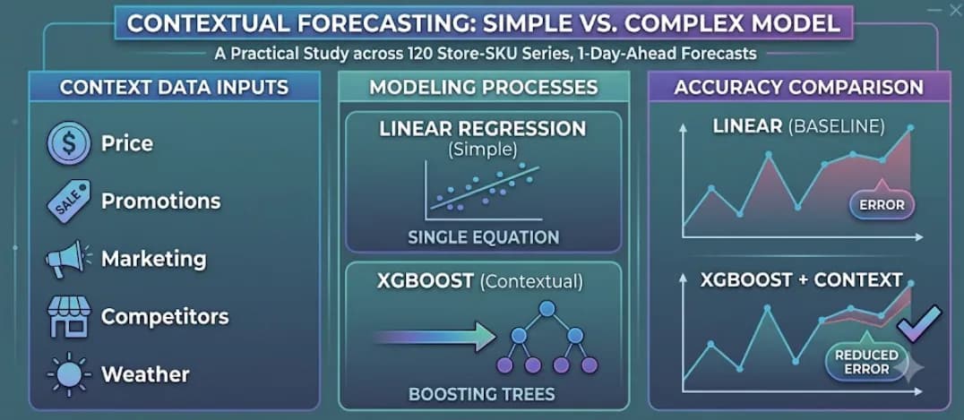
This article continues the case study introduced in Forecasting iPhone 17 Pro Demand: From Statistics to Deep Learning and follows the statistical deep dive, Demand Forecasting with Statistical Models: How Far Can Demand History Alone Take Us?.
The statistical article showed how Holt–Winters and SARIMA could turn one store–SKU demand history into a useful one-day-ahead forecast. In such a setup, each store–SKU combination needs its own fitted model. Twenty stores and six SKUs would therefore require 120 models, each learning its own parameters. This local approach also creates a practical maintenance burden.
Now we change both the scope of the forecasting system and the information available to it. Instead of fitting one model to one demand history, we train global supervised-learning models across 120 related store–SKU series. A global model can share evidence across stores and products, represent nonlinear relationships, and—depending on the experiment—use price, promotions, marketing, competitor activity, and weather alongside demand history and the calendar.
This article is structured as follows:
- The forecasting question changes
- Turn a time series into supervised-learning rows
- Feature engineering creates memory
- Supervised learning
- Model selection
- What feature importance can and cannot say
- Operational recommendation
- What supervised learning costs
The forecasting question changes
The statistical models in the previous experiment answered:
How does demand evolve from its own past?
Holt–Winters represented demand through level, trend, and seasonality. SARIMA modelled relationships between previous values and previous forecast errors. Both extracted substantial predictive information from demand history. However, because demand history was their only input, they could not directly account for information known before the forecast date, such as:
- a promotion would begin tomorrow;
- the price had changed;
- a marketing campaign was active;
- the store would be closed;
- a competitor had launched an offer;
- heavy rain was forecast.
Unlike the local statistical models, the global supervised-learning model is trained on pooled observations from all 120 series, allowing patterns learned from one store or product to inform forecasts for related series.
To a history-only model, an unexpected promotion surge was simply a forecast error.
Supervised learning reframes the problem:
Can one global supervised-learning model share patterns across 120 store–SKU series—and do nonlinear modelling and additional business context improve its held-out forecasts?
For store , SKU , and forecast date , we write:
The feature vector can contain demand history, calendar position, store and SKU identity, and business signals known before begins.
This question separates three ideas: learning across related series, comparing linear and nonlinear models, and testing whether business context adds value beyond demand history and calendar features.
Keep evaluation chronological
To answer the forecasting question fairly, we retain the chronological boundaries used in the statistical experiment. The final 112 days are divided into consecutive 56-day validation and test windows, rather than randomly shuffling observations across time.
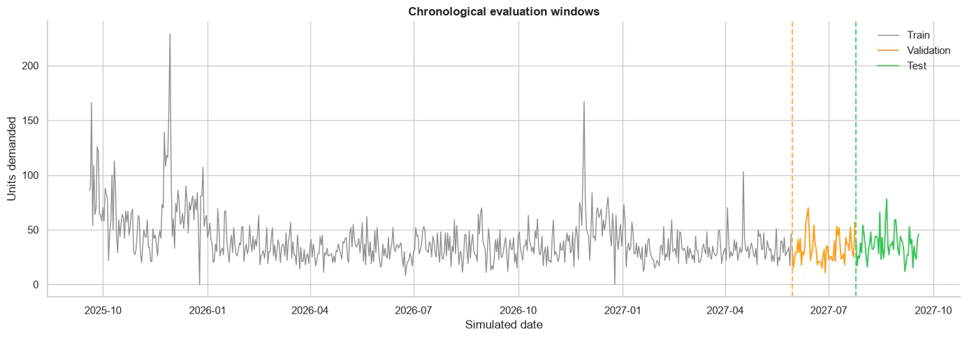
The figure shows one representative store–SKU series, but the same date boundaries are applied to all 120 series. For supervised learning, the first 28 training dates are additionally removed because the lag and rolling features do not yet have sufficient history.
After the 28-day warm-up, the chronological windows contain:
| Window | Days | Panel rows | Purpose |
|---|---|---|---|
| Training | 590 | 70,800 | Estimate relationships |
| Validation | 56 | 6,720 | Select boosting rounds and compare specifications |
| Test | 56 | 6,720 | Evaluate locked models once |
All series share the same date boundaries. Pooling never permits a target from a future date—even from another store—to enter the training set.
Turn a time series into supervised-learning rows
A tabular model has no memory of sequence order. It sees independent rows of features and targets. To use it for forecasting, we must turn the sequence into a supervised-learning table.
For each store–SKU and date, one row contains:
Information available before tomorrow → Tomorrow's demand
An illustrative row might be:
| Feature | Value |
|---|---|
| Demand yesterday | 34 |
| Demand seven days ago | 41 |
| Seven-day average | 36.4 |
| Weekend | Yes |
| Promotion planned | No |
| Store | Example store |
| SKU | Example 256GB SKU |
| Target: tomorrow's demand | 50 |
The target appears in the training table because the historical outcome is known when the model is fitted. It must never appear among the input features for that same row.
The synthetic dataset contains 730 daily observations for each of 120 store–SKU series—20 stores and six SKUs—giving 87,600 rows in total. Our longest historical feature looks back 28 days, so the first 28 observations of each series do not have a complete feature history. Removing this warm-up period leaves 702 observations per series, or 84,240 supervised-learning rows.
Feature engineering creates memory
The statistical models represented temporal structure internally. A tabular model needs us to expose that structure as columns.
Lag features
A lag gives the model an earlier demand value:
Consider four consecutive days from one store–SKU series:
| Date | Observed demand | Lag 1 feature |
|---|---|---|
| Day 1 | 34 | — |
| Day 2 | 41 | 34 |
| Day 3 | 38 | 41 |
| Day 4 | 50 | 38 |
Each lag 1 value is the demand observed one day earlier. For Day 4, the model receives 38 as an input, while 50 is the target and remains unknown when the forecast is produced.
The experiment uses lags of 1, 7, 14, and 28 days:
- lag 1 captures the most recent demand and short-term persistence;
- lag 7 compares the forecast date with the same weekday last week;
- lag 14 checks whether the weekly pattern has persisted for two weeks;
- lag 28 provides a four-week reference that is less sensitive to one unusual week.
Shifted rolling statistics
Rolling means and standard deviations summarise recent level and volatility. For a seven-day mean used to predict date :
The sum ends at . This one-period shift is essential: including would leak the target into its own predictors.
The experiment uses rolling statistics of 7 and 28 days.
Cyclical calendar features
Weekdays and days of the year repeat. Representing weekdays as integers would assign Monday 0 and Sunday 6, creating an artificial distance between two adjacent days. Instead, sine and cosine map their positions onto a circle:
Here, for the weekly cycle and for the annual cycle.
Both are needed because sine alone assigns the same value to more than one position on the circle. The pair uniquely represents position within the weekly or annual cycle.
- Weekly position:
dow_sinanddow_cos - Annual position:
doy_sinanddoy_cos
The history, calendar, and identity feature set ultimately contains 18 numeric features and four categorical fields. The full-context set expands this to 27 numeric features and five categorical fields.
The 18 numeric features are:
| Feature group | Features | Count |
|---|---|---|
| Demand lags | 1, 7, 14, and 28 days | 4 |
| Rolling statistics | Mean and standard deviation over 7 and 28 days | 4 |
| Cyclical calendar | Weekday sine/cosine and annual sine/cosine | 4 |
| Calendar flags | Weekend, public holiday, store open, Black Friday week | 4 |
| Lifecycle | Days since launch | 1 |
| Product attribute | Storage capacity | 1 |
| Total | 18 |
The four categorical fields are store ID, SKU ID, store tier, and colour family. The full-context set adds nine numeric business features—price and discount information, promotion and competitor flags, marketing, and weather—and promotion type as a fifth categorical field. This produces 27 numeric features and five categorical fields before one-hot encoding.
Prevent data leakage
Creating a feature is only half the task. We must also confirm that its value would have been available when the forecast was produced. Otherwise, the model may learn from information that belongs to the future.
Data leakage is not only a coding error; it can also be a business-definition error. A variable may exist in the final dataset without having existed at the forecast timestamp. Realised rainfall, for example, is not a valid input to a forecast created the previous evening—the model would have had access only to the weather forecast available at that time.
The experiment uses the following availability assumptions:
| Feature group | Examples | Day-ahead assumption |
|---|---|---|
| Historical demand | Lags and rolling statistics | Observed through yesterday's close |
| Calendar | Weekday, holiday, closure | Known in advance |
| Static identity | Store, tier, SKU, storage | Known in advance |
| Commercial plan | Price, discount, promotion | Published before the forecast run |
| Marketing | Campaign index | Supplied by the campaign plan |
| Competitor | Competitor promotion flag | Supplied by market monitoring |
| Weather | Temperature and rain | Day-ahead weather forecast |
The synthetic data contain realised values for marketing, competitors, and weather. For this case study, we treat them as perfectly available day-ahead signals. That assumption is deliberately optimistic.
In a production backtest, each input should come from the point-in-time snapshot that genuinely existed at the forecast timestamp. Replacing a historical weather forecast with observed weather would quietly make the model look better than it could have been in operation.
The rule is simple:
A feature is valid only if its value, source, owner, and availability time are known before the prediction is made.
Prepare features for modelling
Before training, the numeric and categorical features must be converted into a model-ready matrix.
| Feature type | Preprocessing | Purpose |
|---|---|---|
| Numeric | Standardisation | Centres each feature around zero and scales it by its training-set standard deviation |
| Categorical | One-hot encoding | Creates a binary column for each category without imposing an artificial order |
Standardisation is particularly useful for linear regression because its inputs may have very different scales—for example, storage capacity, price, and rainfall. Tree-based XGBoost does not require scaled numeric features.
Store, SKU, tier, colour family, and promotion type are one-hot encoded. For
example, store_id becomes a collection of store-specific indicator columns
rather than an integer that would incorrectly imply an order between stores.
Most importantly, the preprocessor is fitted only on the training data. Its learned means, standard deviations, and categories are then applied unchanged to validation data. This prevents preprocessing itself from leaking future information.
Supervised learning
The experiment uses two supervised-learning model families. Linear regression provides an interpretable baseline; XGBoost provides nonlinear interactions and greater flexibility.
Linear regression
Linear regression estimates tomorrow's demand as a weighted sum of features:
An illustrative forecast might be:
Baseline demand              25 units
Strong demand last week      +8 units
Weekend                      +6 units
Promotion                    +4 units
Higher price                 −3 units
Competitor promotion         −2 units
------------------------------------------------
Predicted demand             38 units
The model is fast and easy to inspect. It reveals whether simple additive relationships already explain the target.
That simplicity comes with several assumptions and limitations:
1. Linearity and additivity.
Linear regression assumes that expected demand can be represented as a weighted sum of the supplied features. Without additional terms, a discount receives the same marginal effect across stores, products, and calendar conditions. Nonlinear or non-additive relationships can be introduced through engineered features.
To make the promotion effect different on weekends, for example, we would need a feature such as:
These terms make the relationship nonlinear in the original inputs, but the regression remains linear in its coefficients. The limitation is that the modeller must decide which interactions and transformations to include; linear regression does not discover them automatically.
2. Multicollinearity.
Features such as price, discount, promotion status, and promotion type may contain overlapping information. Strongly correlated features can make individual coefficients unstable, even when the resulting predictions remain similar. Typical remedies include removing redundant variables, selecting a reference category during one-hot encoding, or using regularisation such as Ridge regression. Standardisation puts features on comparable scales, but it does not remove multicollinearity.
3. Error behaviour.
Classical regression analysis assumes that the remaining errors have no systematic relationship with the inputs, have reasonably stable variance, and are not strongly correlated across observations. Time-series errors may violate these conditions because neighbouring dates share demand patterns and high-demand periods may produce larger errors. Normal residuals are mainly needed for conventional statistical tests and analytical intervals, not for calculating point forecasts.
In this experiment, linear regression is used as a predictive baseline rather than for causal interpretation, coefficient significance tests, or analytical prediction intervals. We therefore do not need to correct every violation for statistical inference. Instead, we assess whether the model generalises through its chronological validation and test performance. The assumptions still matter when their violation reduces forecast accuracy, but their practical effect is judged through MAE, RMSE, WAPE, and bias rather than through coefficient -values. If coefficient stability became important in production, Ridge regression and residual diagnostics would be sensible extensions.
XGBoost
Unlike linear regression, XGBoost can learn nonlinear relationships, thresholds, and feature interactions directly from the data. A decision tree begins with all training observations in one group. At each node, it tests possible features and thresholds, then selects the split that produces the largest reduction in prediction error.
XGBoost builds an ensemble of decision trees sequentially. The first tree improves an initial prediction. Each later tree focuses on where the current ensemble still incurs loss.
The final prediction is the sum of many small corrections:
where is tree , is the number of trees, and is the learning rate controlling how much each tree contributes.
Under squared-error loss, the negative gradient is proportional to the residual:
This is why boosting is often described as repeatedly learning the remaining errors. More generally, XGBoost uses the first and second derivatives of its objective to evaluate efficient split improvements.
A simplified sequence might look like:
Initial prediction                    40
Tree 1: lifecycle adjustment          −5
Tree 2: weekend interaction           +7
Tree 3: promotion-weekend interaction +6
Tree 4: recent-demand correction      +3
------------------------------------------------
Final forecast                        51
Individual trees are not normally interpretable as clean business effects like this; the example only illustrates how corrections accumulate.
Tree splits naturally represent thresholds and interactions. A discount can matter only after it exceeds 10%, heavy rainfall can matter more than light rain, and a promotion can behave differently by store, SKU, weekday, and lifecycle stage without manually defining every combination.
That flexibility needs control. The experiment uses shallow-enough trees, learning-rate shrinkage, row and feature subsampling, L1 and L2 regularisation, and early stopping. Training stops when validation MAE fails to improve for 50 rounds. The history, calendar, and identity model selects 529 trees, while the full-context model selects 289. Those counts are then locked before the test window is opened.
Model selection
The experiment evaluates three global model configurations through two controlled comparisons. WAPE remains the primary metric, aggregated across all 120 store–SKU series. Validation guides model development; the locked test window shows whether those choices generalise.
Compare model structures
Objective. Determine whether a tree-based model improves forecasting when both models receive exactly the same information.
Controlled design. Full-context linear regression and full-context XGBoost use the same history, calendar, and business features, as well as the same chronological training, validation, and test windows. The main difference is model structure: linear regression uses predefined additive relationships, whereas XGBoost learns thresholds and interactions.
Performance. WAPE remains the primary metric, aggregated across all 120 store–SKU series.
| Model | Validation WAPE | Test WAPE |
|---|---|---|
| Linear regression: full context | 27.75% | 27.17% |
| XGBoost: full context | 26.72% | 26.62% |
XGBoost improves test WAPE by 0.55 percentage points. This suggests that the more flexible tree structure adds predictive value beyond the additive model, although the improvement is modest rather than transformational.
Evaluate additional business context
Objective. Determine whether price, promotions, marketing, competitor activity, and weather improve XGBoost beyond demand history and calendar information.
Controlled design. Both configurations use XGBoost and the same global training process. The core model sees lags, rolling statistics, calendar fields, and store and product identity. The full-context model adds the business signals. Only the information set changes, making this a group-level ablation rather than individual feature selection.
Performance. Validation initially favours the richer model, but the locked test result changes the conclusion.
| Model | Validation WAPE | Test WAPE |
|---|---|---|
| XGBoost: history, calendar, and identity | 27.13% | 26.60% |
| XGBoost: full business context | 26.72% | 26.62% |
Additional context improves validation WAPE by 0.41 percentage points but does not improve test WAPE. The 0.02-point test difference is negligible, so the two models are effectively tied on the primary metric. The full-context model has a lower test RMSE—6.48 versus 6.64—but its extra forecast-time dependencies are not justified by WAPE alone.
Their biases also point in opposite directions: the core XGBoost model underforecasts by 4.91% in aggregate, while full-context XGBoost overforecasts by 2.30%. Model selection therefore depends on more than ranking a single accuracy number.
This does not prove that promotions, price, marketing, competitors, and weather are useless. The 56-day test window may represent a different regime, some context variables may duplicate information already contained in demand history, and the synthetic signals may be noisy relative to daily store–SKU variation. Importance and a single holdout cannot complete feature selection; incremental value should be checked across additional rolling validation windows.
Selection outcome
The evidence supports XGBoost over the additive linear baseline. It does not show a stable WAPE benefit from the additional business-context feature group. The simpler history, calendar, and identity configuration is therefore an operationally attractive candidate, but that choice remains provisional until it is confirmed across more rolling validation periods and a new untouched evaluation window.
What feature importance can and cannot say
Gain-based feature importance measures how much a feature reduced XGBoost's regularised training objective across tree splits. Every time XGBoost builds a tree, it evaluates possible splits. A split is useful when dividing the observations into two groups reduces the model’s regularised training objective.
In simplified form:
Suppose a tree node contains observations with a training loss of 1,000.
Splitting those observations using is_black_friday_week reduces the combined loss of the two resulting branches to 700:
That split contributes a gain of 300 to is_black_friday_week. XGBoost repeats this process across every node and every tree.
The gains from all splits using the same feature are then added together:
The importances are then normalised.
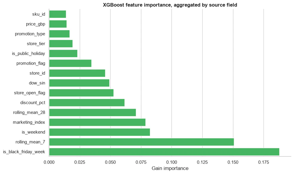
For the full-context model, the leading fields include:
- Black Friday week: 18.8%;
- seven-day rolling mean: 15.1%;
- weekend: 8.2%;
- marketing index: 7.9%;
- 28-day rolling mean: 7.1%;
- discount percentage: 6.2%.
This looks like evidence that context matters. But importance answers a training question, not a deployment question. It says the model used a feature to reduce its fitted objective. It does not say that the feature caused demand, would survive a policy change, or improved held-out accuracy.
Correlated features can substitute for one another. Store identity can absorb information associated with store tier; price can overlap with discount and promotion type. A field with low individual importance may still matter through interactions, while a field with high importance may fail to generalise.
The most important evidence remains the controlled context comparison: the full-context model did not beat the core model on test. Feature importance cannot overturn that result.
Operational recommendation
Treat history, calendar, and identity XGBoost as the provisional leading candidate for the global forecasting system. It achieves the lowest held-out panel WAPE and requires fewer forecast-time dependencies, but its 0.02-percentage-point advantage over full-context XGBoost is negligible. Confirm the choice across additional rolling validation periods and a new untouched evaluation window before treating it as final.
Retain full-context XGBoost, global linear regression, and seasonal naive as challengers. They provide useful reference points for detecting whether the core model has stopped adding value. Its 4.91% aggregate underforecasting bias should also be monitored rather than hidden behind its leading WAPE.
Before promoting the full-context model:
- reconstruct every feature from genuine point-in-time sources;
- evaluate across additional rolling windows and business regimes;
- verify performance during promotions, holidays, launches, and competitor events;
- measure stockouts and excess inventory alongside WAPE and bias;
- add an uncertainty method if the forecast will set service levels or safety stock.
Each daily model run should generate one demand forecast for every store–SKU series. These predictions are demand baselines, not order quantities. Replenishment must still account for stock on hand, confirmed inbound inventory, lead time, and the chosen safety buffer.
What supervised learning costs
Supervised learning expands what the model can represent, but it also expands what the forecasting system must maintain.
- Feature pipelines create memory. Every lag and rolling statistic must be computed consistently in training and production.
- Availability rules prevent leakage. Every future covariate needs a point-in-time source and an accountable owner.
- Global training shares evidence. One model can learn across stores and products, but identity features and distribution shifts must be monitored.
- Flexible models can overfit. Early stopping and regularisation reduce the risk; held-out time windows reveal whether they succeeded.
- Importance is not causality. A model using a feature does not prove that changing the feature will change demand.
- Uncertainty is not automatic. Calibrated intervals require an additional method such as conformal prediction, quantile objectives, or a probabilistic model.
The experiment answers its title with a qualified result. Supervised learning helped: both XGBoost models improved global panel WAPE over linear regression and seasonal naive. More context did not help global test WAPE: the fuller information set failed to generalise better on the article's primary metric, although it achieved a slightly lower RMSE.
That is not a disappointing conclusion. It is exactly why we use chronological validation, ablation tests, and honest holdouts. A feature earns its operational cost only when it improves decisions outside the data used to choose it.
這篇文章延續了 預測 iPhone 17 Pro 需求:從統計方法到深度學習 中介紹的案例研究,並接續統計深度解析文章 僅憑歷史需求,我們能預測到多準?。
前一篇文章說明 Holt-Winters 與 SARIMA 如何利用單一門市-SKU 的需求歷史產生隔日預測。在這種局部建模架構下,每個組合都要分別配適模型;20 家門市與 6 個 SKU 便需要維護 120 個模型與各自的參數。
本次實驗同時擴大建模範圍與可用資訊,不再為每條序列個別配適模型,而是以 120 條相關的門市-SKU 序列訓練全域監督式模型。全域模型可以跨門市與產品共享統計訊號、表示非線性關係,並視實驗設定,在需求歷史與日曆之外加入價格、促銷、行銷、競品動態與天氣資訊。
本文架構如下:
1. 預測問題的改變
前一個實驗中的統計模型,回答的是:
需求如何從自己的過去演變而來?
Holt-Winters 透過水準、趨勢與季節性來表示需求;SARIMA 則對過去數值與過去預測誤差之間的關係建模。兩者都從需求歷史中,萃取出相當豐富的預測資訊。然而,由於需求歷史是它們唯一的輸入,它們無法直接納入在預測日期之前就已經得知的資訊,例如:
- 明天將展開一項促銷活動;
- 價格已經改變;
- 行銷活動正在進行;
- 門市即將公休;
- 競爭對手推出了優惠;
- 預報將有大雨。
與局部的統計模型不同,全域監督式學習模型是用全部 120 條序列彙整而成的觀測值來訓練,讓從某一家門市或某項產品學到的模式,能夠用來輔助相關序列的預測。
對於一個只看歷史的模型而言,一次未預期的促銷激增,就只是一次預測誤差。
監督式學習重新界定了這個問題:
一個全域監督式學習模型,能不能在 120 條門市-SKU 序列之間共享模式?非線性建模與額外的商業情境資訊,是否能改善它在保留樣本上的預測表現?
對於門市 、SKU 與預測日期 ,我們可以寫成:
特徵向量 可以包含需求歷史、日曆位置、門市與 SKU 身分,以及在 開始之前就已得知的商業訊號。
這個問題把三個概念區分開來:跨相關序列學習、比較線性與非線性模型,以及測試商業情境資訊,是否能在需求歷史與日曆特徵之外,帶來額外的價值。
維持依時間順序的評估方式
為了公平地回答這個預測問題,我們沿用統計實驗中所使用的時間邊界。最後 112 天被劃分成連續的 56 天驗證區間與 56 天測試區間,而不是把觀測值跨時間隨機打亂。
這張圖顯示的是一條具代表性的門市-SKU 序列,但相同的日期邊界,會套用到全部 120 條序列上。在監督式學習中,訓練集最前面的 28 天會被額外移除,因為此時落後特徵與滾動特徵,還沒有足夠的歷史資料可用。
經過 28 天的暖身期之後,依時間順序劃分的區間包含:
| 區間 | 天數 | 追蹤資料列數 | 用途 |
|---|---|---|---|
| 訓練集 | 590 | 70,800 | 估計模型參數與關係 |
| 驗證集 | 56 | 6,720 | 選擇提升回合數並比較不同規格 |
| 測試集 | 56 | 6,720 | 僅評估一次已鎖定的模型 |
所有序列共用相同日期邊界。資料整理流程不得讓未來日期的目標值進入訓練特徵。
2. 把時間序列轉換成監督式學習的資料列
表格型模型不會自行保留序列順序;它接收的是一列列特徵與目標值。因此,必須先把時間序列轉換為監督式學習表格。
對每一個門市-SKU 與日期組合而言,一列資料包含:
明天之前可取得的資訊 → 明天的需求
一列示意資料可能如下:
| 特徵 | 數值 |
|---|---|
| 昨天的需求 | 34 |
| 七天前的需求 | 41 |
| 七天平均 | 36.4 |
| 是否為週末 | 是 |
| 是否計畫促銷 | 否 |
| 門市 | 示範門市 |
| SKU | 示範 256GB SKU |
| 目標:明天的需求 | 50 |
目標值之所以會出現在訓練表格中,是因為在配適模型時,這個歷史結果已經是已知的。但它絕不能出現在同一列的輸入特徵之中。
這個合成資料集,為 120 條門市-SKU 序列——20 家門市乘以 6 個 SKU——各自提供 730 筆每日觀測值,總共 87,600 列。我們最長的歷史特徵回顧 28 天,因此每條序列最前面的 28 筆觀測值,都沒有完整的特徵歷史可用。移除這段暖身期之後,每條序列剩下 702 筆觀測值,也就是 84,240 列監督式學習資料。
3. 特徵工程為模型建立時間記憶
統計模型在內部表示時間結構;表格型模型則需要把這些結構明確轉換為欄位。
落後特徵
落後特徵,會提供模型一個更早期的需求值:
考慮某條門市-SKU 序列中連續四天的資料:
| 日期 | 觀測需求 | 落後 1 期特徵 |
|---|---|---|
| 第 1 天 | 34 | — |
| 第 2 天 | 41 | 34 |
| 第 3 天 | 38 | 41 |
| 第 4 天 | 50 | 38 |
每一個 落後 1 期 的數值,都是一天前觀測到的需求。以第 4 天為例,模型接收到的輸入是 38,而 50 則是目標值,在產生預測時仍屬未知。
這項實驗使用落後 1、7、14 與 28 天的特徵:
- 落後 1 期 捕捉最近期的需求與短期持續性;
- 落後 7 期 把預測日期,與上週同一個星期幾相比;
- 落後 14 期 檢查每週模式是否已經持續了兩週;
- 落後 28 期 提供一個四週的參考基準,對單一一週的異常較不敏感。
位移後的滾動統計量
滾動平均與滾動標準差,用來彙總近期的水準與波動性。以用來預測日期 的七天平均為例:
這個加總截至 。位移非常重要:若納入 ,目標值就會洩漏到用來預測自身的特徵中。
這項實驗使用 7 天與 28 天的滾動統計量。
週期性日曆特徵
星期幾與一年中的日子,都是重複出現的。如果用整數表示星期幾,星期一是 0、星期日是 6,就會在兩個相鄰的日子之間,製造出人為的距離。因此,這裡改用正弦與餘弦,把它們的位置對應到一個圓上:
其中,每週週期的 ,年度週期的 。
兩者都需要,是因為單靠正弦,會把同一個數值指派給圓上不只一個位置。正弦與餘弦成對使用,才能唯一地表示在每週或年度週期中的位置。
- 每週位置:
dow_sin與dow_cos - 年度位置:
doy_sin與doy_cos
「歷史、日曆與身分」這組特徵集合,最終包含 18 個數值特徵與 4 個類別欄位。「完整情境」特徵集合,則將其擴充為 27 個數值特徵與 5 個類別欄位。
這 18 個數值特徵為:
| 特徵群組 | 特徵內容 | 數量 |
|---|---|---|
| 需求落後特徵 | 1、7、14、28 天 | 4 |
| 滾動統計量 | 7 天與 28 天的平均與標準差 | 4 |
| 週期性日曆 | 星期幾的正弦/餘弦,以及年度的正弦/餘弦 | 4 |
| 日曆旗標 | 週末、國定假日、門市是否營業、黑色星期五週 | 4 |
| 生命週期 | 距離上市天數 | 1 |
| 產品屬性 | 儲存容量 | 1 |
| 總計 | 18 |
這 4 個類別欄位分別是門市編號、SKU 編號、門市等級與色系。「完整情境」特徵集合,再加上 9 個數值商業特徵——價格與折扣資訊、促銷與競爭對手旗標、行銷與天氣——以及作為第五個類別欄位的促銷類型。在進行 one-hot 編碼之前,總共會產生 27 個數值特徵與 5 個類別欄位。
避免資料洩漏
建立特徵只是第一步,還必須確認它在預測時間點確實可取得,否則模型可能從未來資訊中學習。
資料洩漏不只是程式碼上的錯誤,也可能是業務定義上的錯誤。一個變數,可能存在於最終的資料集中,卻在預測產生的當下並不存在。舉例來說,實際發生的降雨量,並不是前一天晚上產生預測時的有效輸入——模型當時所能取得的,只有在那個時間點可用的天氣預報。
這項實驗採用以下的可取得性假設:
| 特徵群組 | 範例 | 隔日可取得性假設 |
|---|---|---|
| 歷史需求 | 落後特徵與滾動統計量 | 觀測至昨天收盤為止 |
| 日曆 | 星期幾、假期、公休 | 事先已知 |
| 靜態身分 | 門市、等級、SKU、容量 | 事先已知 |
| 商業計畫 | 價格、折扣、促銷 | 在預測執行前已公布 |
| 行銷 | 活動指數 | 由行銷活動計畫提供 |
| 競爭對手 | 競爭對手促銷旗標 | 由市場監測提供 |
| 天氣 | 氣溫與降雨 | 隔日天氣預報 |
合成資料中的行銷、競品與天氣欄位是事件發生後的實際值。本案例假設這些值能在隔日預測前完整取得,屬於刻意採用的樂觀設定。
正式環境的回測必須使用預測當下確實存在的即時時點快照。若以事後觀測天氣取代當時的歷史天氣預報,評估結果就會高估實際可達成的表現。
這條規則很簡單:
唯有當一個特徵的數值、來源、負責人與可取得時間,都在做出預測之前就已確定,這個特徵才是有效的。
為建模準備特徵
在訓練之前,數值與類別特徵,都必須轉換成模型可用的矩陣形式。
| 特徵類型 | 前處理方式 | 目的 |
|---|---|---|
| 數值 | 標準化 | 將每個特徵置中在零附近,並依訓練集的標準差進行縮放 |
| 類別 | One-hot 編碼 | 為每個類別建立一個二元欄位,不強加人為的順序關係 |
標準化對線性迴歸特別有用,因為它的輸入可能有相當不同的尺度——例如儲存容量、價格與降雨量。以樹為基礎的 XGBoost,則不需要經過縮放的數值特徵。
門市、SKU、等級、色系與促銷類型,都會經過 one-hot 編碼。舉例來說,store_id 會變成一組門市專屬的指標欄位,而不是一個會錯誤暗示門市之間存在順序關係的整數。
最重要的是,前處理器只在訓練資料上配適。它學到的平均數、標準差與類別,接著會原封不動地套用到驗證資料上。這樣可以避免前處理本身,洩漏了未來的資訊。
4. 監督式學習
這項實驗使用兩種監督式學習模型家族。線性迴歸提供一個可解釋的基準模型;XGBoost 則提供非線性交互作用與更高的彈性。
線性迴歸
線性迴歸把明天的需求,估計為特徵的加權總和:
一個示意性的預測可能如下:
基準需求                     25 台
上週需求強勁                 +8 台
週末                         +6 台
促銷                         +4 台
價格較高                     −3 台
競爭對手促銷                 −2 台
------------------------------------------------
預測需求                     38 台
這個模型速度快,也容易檢視。它能顯示出簡單的加法關係,是否就已經能解釋目標值。
這種簡單性,也伴隨著幾項假設與限制:
1. 線性與可加性。
線性迴歸假設,預期需求可以表示成所提供特徵的加權總和。在沒有額外項的情況下,折扣在不同門市、產品與日曆條件下,都會產生相同的邊際效應。非線性或非可加性的關係,則可以透過工程設計出來的特徵來引入。
舉例來說,如果想讓促銷效應在週末有所不同,我們就需要一個像這樣的特徵:
這類項目,會讓關係在原始輸入上呈現非線性,但迴歸本身在係數上仍然是線性的。它的限制在於:建模者必須自行決定要納入哪些交互作用與轉換;線性迴歸並不會自動發現這些關係。
2. 共線性。
價格、折扣、促銷狀態與促銷類型等特徵,可能包含重疊的資訊。高度相關的特徵,即使最終預測結果相近,也可能讓個別係數變得不穩定。常見的因應方式包括:移除多餘的變數、在 one-hot 編碼時選定一個參照類別,或使用像 Ridge 迴歸 這樣的正則化方法。標準化能讓特徵處於可比較的尺度上,但並不能消除共線性。
3. 誤差行為。
傳統的迴歸分析假設,剩餘的誤差與輸入之間沒有系統性的關係、變異數大致穩定,且觀測值之間不存在強烈的相關性。時間序列的誤差,可能違反這些條件,因為相鄰的日期會共享需求模式,而需求量高的期間,也可能產生較大的誤差。常態分布的殘差,主要是傳統統計檢定與解析式區間所需要的,而不是計算點預測所必要的。
在這項實驗中,線性迴歸是作為預測用的基準模型,而不是用於因果推論、係數顯著性檢定,或解析式的預測區間。因此,我們不需要為了統計推論,去修正每一項違反假設的情況。取而代之的是,我們透過依時間順序的驗證與測試表現,來評估模型是否具備泛化能力。當違反這些假設會降低預測準確度時,這些假設仍然重要,但它們的實際影響,是透過 MAE、RMSE、WAPE 與偏差來判斷,而不是透過係數的 值。如果係數的穩定性在正式上線後變得重要,Ridge 迴歸與殘差診斷,會是合理的延伸做法。
XGBoost
與線性迴歸不同,XGBoost 能直接從資料中,學習非線性關係、門檻值與特徵交互作用。一棵決策樹一開始,會把所有訓練觀測值視為同一個群組。在每一個節點上,它會測試可能的特徵與門檻值,接著選出能讓預測誤差降低最多的切分方式。
XGBoost 會依序建立一組決策樹的集成。第一棵樹會改善初始的預測值,之後每一棵樹,都聚焦在目前集成模型仍然產生損失的地方。
最終的預測,就是許多微小修正值的總和:
其中, 是第 棵樹, 是樹的總數,而 則是學習率,控制每一棵樹的貢獻程度。
在平方誤差損失下,負梯度與殘差成正比:
這就是為什麼提升法(boosting)常被描述成「反覆學習剩餘的誤差」。更一般地說,XGBoost 會利用目標函數的一階與二階導數,來有效評估切分所帶來的改善。
一個簡化過的流程可能如下:
初始預測                              40
第 1 棵樹:生命週期調整               −5
第 2 棵樹:週末交互作用               +7
第 3 棵樹:促銷×週末交互作用          +6
第 4 棵樹:近期需求修正               +3
------------------------------------------------
最終預測                              51
個別樹通常無法如此直接地對應特定商業效應;這個例子只用來說明修正值如何累積。
樹的切分,天生就能表示門檻值與交互作用。折扣可能要超過 10% 才會產生影響、大雨的影響可能比小雨更明顯,而促銷在不同門市、SKU、星期幾與生命週期階段中,也可能有不同的表現——而這一切都不需要我們手動定義每一種組合。
這種彈性需要加以控制。這項實驗使用了足夠淺的樹、學習率縮減、資料列與特徵抽樣、L1 與 L2 正則化,以及提前停止。當驗證集 MAE 連續 50 個回合都沒有改善時,訓練就會停止。「歷史、日曆與身分」模型選出了 529 棵樹,而「完整情境」模型則選出了 289 棵樹。這些數量,會在打開測試區間之前先行鎖定。
5. 模型選擇
這項實驗透過兩組控制比較,評估三種全域模型設定。WAPE 仍然是彙總全部 120 條門市-SKU 序列後的主要指標。驗證集用來引導模型開發;已鎖定的測試區間,則用來檢視這些選擇是否能夠泛化。
比較模型結構
目的。 在兩個模型接收到完全相同資訊的前提下,判斷以樹為基礎的模型,是否能改善預測表現。
控制設計。 「完整情境」線性迴歸與「完整情境」XGBoost,使用相同的歷史、日曆與商業特徵,也使用相同的依時間順序劃分之訓練、驗證與測試區間。兩者主要的差異在於模型結構:線性迴歸使用預先定義好的加法關係,而 XGBoost 則會學習門檻值與交互作用。
表現。 WAPE 仍然是彙總全部 120 條門市-SKU 序列後的主要指標。
| 模型 | 驗證集 WAPE | 測試集 WAPE |
|---|---|---|
| 線性迴歸:完整情境 | 27.75% | 27.17% |
| XGBoost:完整情境 | 26.72% | 26.62% |
XGBoost 使測試集 WAPE 降低 0.55 個百分點,顯示樹模型的非線性與交互作用在加法線性模型之外提供了額外預測價值,但改善幅度有限。
評估額外的商業情境資訊
目的。 判斷價格、促銷、行銷、競爭對手動態與天氣,是否能在需求歷史與日曆資訊之外,進一步改善 XGBoost 的表現。
控制設計。 兩種設定都使用 XGBoost,並採用相同的全域訓練流程。核心模型只看得到落後特徵、滾動統計量、日曆欄位,以及門市與產品身分;完整情境模型,則額外加上商業訊號。唯一改變的是資訊集合本身,因此這是一種群組層級的消融測試,而不是逐一特徵篩選。
表現。 一開始,驗證集的結果偏向資訊更豐富的模型,但已鎖定的測試結果,改變了這個結論。
| 模型 | 驗證集 WAPE | 測試集 WAPE |
|---|---|---|
| XGBoost:歷史、日曆與身分 | 27.13% | 26.60% |
| XGBoost:完整商業情境 | 26.72% | 26.62% |
額外情境資訊使驗證集 WAPE 降低 0.41 個百分點,卻未改善測試集 WAPE。測試差異只有 0.02 個百分點,在主要指標上可視為相當。完整情境模型的測試集 RMSE 較低(6.48 對 6.64),但目前證據不足以證明新增資料來源與預測時點相依性具有穩定價值。
兩者的偏差方向也恰好相反:核心 XGBoost 模型整體上低估了 4.91%,而完整情境 XGBoost,則整體上高估了 2.30%。因此,模型選擇所仰賴的,不只是替單一準確度數字排名而已。
這並不代表促銷、價格、行銷、競爭對手與天氣是沒有用的。56 天的測試區間,可能代表著一種不同的狀態;部分情境變數,可能與需求歷史中已經包含的資訊重複;而這些合成訊號,相對於每日門市-SKU 的變動,也可能帶有雜訊。單靠特徵重要性與單一次的保留測試,並不足以完成特徵選擇——增量價值,應該透過額外的滾動驗證區間來檢驗。
選擇結果
現有證據支持 XGBoost 優於加法線性基準,但未顯示額外商業情境特徵能穩定改善 WAPE。因此,較簡單的「歷史、日曆與身分」設定是目前較合理的候選方案;這項選擇仍需透過更多滾動驗證與全新評估區間確認。
6. 特徵重要性能說明什麼、不能說明什麼
以增益為基礎的特徵重要性,衡量的是一個特徵,在所有樹的切分中,總共讓 XGBoost 正則化訓練目標函數降低了多少。每當 XGBoost 建立一棵樹時,都會評估可能的切分方式。當把觀測值切成兩組,能降低模型的正則化訓練目標函數時,這個切分就是有用的。
以簡化的形式表示:
假設某個樹節點中的觀測值,訓練損失為 1,000。使用 is_black_friday_week 來切分這些觀測值後,兩個分支合計的損失降為 700:
這次切分,為 is_black_friday_week 貢獻了 300 的增益。XGBoost 會在每一個節點、每一棵樹上,重複這個流程。接著,把使用同一個特徵的所有切分增益加總起來:
接著,這些重要性數值會經過標準化。
在完整情境模型中,排名最前面的欄位包括:
- 黑色星期五週:18.8%;
- 七天滾動平均:15.1%;
- 週末:8.2%;
- 行銷指數:7.9%;
- 28 天滾動平均:7.1%;
- 折扣百分比:6.2%。
這些結果只能說明模型在訓練期間使用了哪些特徵來降低目標函數,不能證明特徵造成需求變化、在政策改變後仍然有效,或必然改善保留樣本的準確度。
彼此相關的特徵,可以互相替代。門市身分,可以吸收與門市等級相關的資訊;價格,則可能與折扣及促銷類型重疊。一個個別重要性偏低的欄位,仍可能透過交互作用而發揮作用;而一個重要性偏高的欄位,也可能無法順利泛化。
最重要的證據,仍然是那組控制情境比較:完整情境模型,在測試集上並沒有勝過核心模型。特徵重要性,無法推翻這項結果。
7. 營運建議
目前可將「歷史、日曆與身分」XGBoost 視為全域預測系統的主要候選。它在保留樣本上取得最低的彙總 WAPE,且依賴的即時資料來源較少;不過,它相對完整情境 XGBoost 的 0.02 個百分點優勢可以忽略。在定案前,仍應以更多滾動驗證與全新評估區間確認。
應該保留完整情境 XGBoost、全域線性迴歸,以及季節性單純法,作為挑戰模型。它們能提供有用的參照基準,幫助偵測核心模型是否已經不再帶來額外價值。它整體 4.91% 的低估偏差,也應該持續監控,而不是被它領先的 WAPE 表現所掩蓋。
在將完整情境模型升級為正式模型之前:
- 使用真正的即時時點資料來源重建每個特徵;
- 在更多滾動區間與不同的商業狀態下進行評估;
- 驗證在促銷、假期、新品上市與競爭對手事件期間的表現;
- 在 WAPE 與偏差之外,同時衡量缺貨與庫存過剩的情況;
- 如果這個預測將用來設定服務水準或安全庫存,就需要加上一套不確定性方法。
每天執行模型時,都應該為每一條門市-SKU 序列,產生一個需求預測。這些預測是需求基準值,而不是訂購數量。補貨決策,仍然必須將現有庫存、已確認到貨量、前置時間,以及所選定的安全緩衝,都納入考量。
8. 監督式學習的成本
監督式學習擴大了模型所能表示的範圍,但也擴大了預測系統必須維護的範圍。
- 特徵管線為模型建立時間記憶。 每個落後特徵與滾動統計量,都必須在訓練與正式環境中以一致方式計算。
- 可取得性規則能避免資料洩漏。 每一個關於未來的共變數,都需要一個即時時點的來源,以及一位負責任的所有者。
- 全域訓練能共享證據。 單一模型可以跨門市與產品學習,但身分特徵與分布飄移,都必須持續監控。
- 高彈性模型可能過度配適。 提前停止與正則化能降低風險;保留的未見時間區間則用來驗證這些控制是否有效。
- 重要性不等於因果關係。 模型使用了某個特徵,並不能證明改變這個特徵,就會改變需求。
- 不確定性不會自動出現。 校準良好的預測區間,需要額外的方法,例如共形預測(conformal prediction)、分位數目標函數,或機率模型。
實驗得到一個審慎的結論:兩個 XGBoost 模型在彙總 WAPE 上都優於線性迴歸與季節性單純法,顯示監督式學習具有增量價值;但加入更多情境資訊並未改善測試集 WAPE,雖然 RMSE 略低,仍不足以證明其泛化表現更好。
這也說明依時間順序的驗證、消融測試與獨立保留區間為何重要。只有當特徵能在開發資料之外持續改善預測與決策時,新增資料來源所帶來的營運成本才有合理依據。