LLM Fine-Tuning: Teaching a Small Model to Analyze 10-K Risk DisclosuresLLM 微調實務:以小型模型分析 10-K 風險揭露
A practical guide to supervised fine-tuning, PEFT, LoRA, and QLoRA—covering dataset design, loss masking, leakage-resistant evaluation, and a hands-on experiment with SEC 10-K risk disclosures.從監督式微調、PEFT、LoRA 與 QLoRA 出發,說明資料集設計、損失遮罩與防止資料外洩的評估方法,並以 SEC 10-K 風險揭露進行實驗。
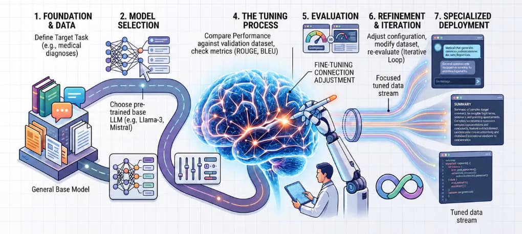
Fine-tuning adapts a pretrained model to reproduce one specific behavior. The hard part isn't starting the training job — it's deciding what that behavior should be, building examples that express it consistently, and proving the resulting adapter actually beats a well-prompted baseline.
This article is organized into four parts:
- Part I: Fine-Tuning Overview
- Part II: LoRA and QLoRA
- Part III: Evaluating a Fine-Tuned Model
- Part IV: Hands-On SEC 10-K Risk-Analysis Case
This article assumes familiarity with decoder-only Transformers — see LLM Pretrain: Anatomy of a Decoder-Only Transformer for background.
Part I: Fine-Tuning Overview
Fine-tuning is useful when a desired behavior is repeated, specific, and difficult to obtain reliably through prompting alone. It is an optimization step, not an automatic first step.
Is Fine-Tuning the Right Tool?
Before investing compute and time into training, it is crucial to establish a strong baseline using few-shot prompting or Retrieval-Augmented Generation (RAG). Prompting injects facts and context, whereas fine-tuning alters a model's fundamental tone, structure, and reasoning pathways.
You should consider moving from prompting to fine-tuning when:
- You are consistently maxing out your context window with complex, highly specific few-shot examples.
- You require rigid, guaranteed output formats (such as a strict JSON schema mapping out 10-K risk severities) that prompting alone cannot reliably enforce.
- Cost or latency constraints dictate replacing a massive proprietary model with a smaller, specialized open-weights model (e.g., an 8B parameter model).
| Requirement | Recommended Approach |
|---|---|
| Improve a one-off instruction | Prompt engineering |
| Access current or private documents | Retrieval-augmented generation (RAG) |
| Add frequently changing financial facts | Retrieval-augmented generation (RAG), not model memory |
| Reproduce a stable tone, taxonomy, or output schema | Fine-tuning |
| Teach consistent decisions from labeled examples | Fine-tuning |
| Reproduce a stable tone, taxonomy, or JSON schema | Fine-tuning |
These approaches are complementary; in our 10-K experiment, retrieval supplies the relevant SEC disclosure, while fine-tuning teaches the model exactly how to analyze and format it.
The Supervised Fine-Tuning (SFT) Objective
Fine-tuning encompasses several distinct objectives. A model might undergo continued pretraining for domain terminology, SFT for task behavior, and preference tuning (like DPO or RLHF) to refine its output choices.
Fine-tuning is not a single training objective; it encompasses several distinct methods that teach different kinds of adaptation.
| Method | What it teaches |
|---|---|
| Continued pretraining | Domain language, terminology, and document patterns through next-token prediction |
| Supervised fine-tuning (SFT) | Desired input-to-output behaviour from labelled demonstrations |
| Preference tuning | Which of two responses is preferable, using methods such as Direct Preference Optimisation (DPO) |
| Reinforcement learning | Behaviour that maximises a reward signal, using approaches such as RLHF or RLAIF |
For our 10-K experiment, the primary objective is SFT because our desired output can be expressed as labeled prompt-completion pairs.
The causal language-modeling objective does not fundamentally change from pretraining: the model still predicts the next token. What changes is the data distribution. While raw documents teach the model to merely continue text, curated SFT demonstrations teach it to respond to a specific request in a consistent, structural way.
Chat Templates: The Training Contract
A conversation represented as role and content objects must eventually
become one token sequence. A chat template inserts the control tokens that mark
system, user, assistant, and message boundaries:
Structured messages
        ↓ model-specific chat template
[system control tokens   ]  instruction
[user control tokens     ]  request
[assistant control tokens]  response
        ↓ tokenizer
Training token IDs
Different model families use entirely different control tokens. For example, LLaMA-3 structures its prompts using <|start_header_id|> and <|eot_id|>,
while Mistral uses [INST] and [/INST]. Training and inference must use the exact template associated with the selected tokenizer.
Manually reproducing another model's format will materially degrade response quality.
The transformers library exposes this conversion through tokenizer.apply_chat_template:
from transformers import AutoTokenizer

tokenizer = AutoTokenizer.from_pretrained("mistralai/Mistral-7B-Instruct-v0.1")
chat = [
  {"role": "system", "content": "You are a financial assistant."},
  {"role": "user", "content": "Analyze this 10-K excerpt."},
  {"role": "assistant", "content": "{\"risks\": [...]}"}
]

# This outputs the properly formatted flat string with control tokens
tokenizer.apply_chat_template(chat, tokenize=False)
Hugging Face chat-template guide
Loss Masking: Completion-Only Loss
Once the text is formatted, we must tell the optimizer what to learn. During completion-only training, prompt tokens provide necessary context, but they should not contribute to the loss. We only want to penalize the model for errors in the assistant's response.
We achieve this using a label mask. The ignore value -100 tells the PyTorch cross-entropy implementation not to score those positions:
Tokens: [system instruction] [user prompt] [assistant response]
Labels: [       -100      ] [   -100    ] [ compute loss here ]
By masking the prompt, we concentrate the learning signal entirely on the behavior the model must produce. In current versions of the TRL (Transformer Reinforcement Learning) library,
prompt-completion datasets use completion-only loss by default. Conversational datasets can trigger this behavior using assistant_only_loss=True,
provided the chat template supplies a valid generation mask.
(For implementation details, refer to the TRL SFTTrainer loss-masking documentation)
Training on the full sequence is also a legitimate objective in other settings, so response-only masking should be selected deliberately rather than treated as a universal rule.
Full Fine-Tuning vs. PEFT
Full fine-tuning updates every parameter in the model, demanding massive memory for gradients and optimizer states. Every specialized model requires storing a complete set of multi-gigabyte weights.
Parameter-efficient fine-tuning (PEFT) freezes most of the base model and trains a fraction of the parameters. The industry standard taxonomy divides PEFT into three high-level strategies:
| PEFT Strategy | Mechanism | Representative Methods |
|---|---|---|
| Additive | Freezes the base model and introduces new trainable parameters. | Adapter modules, prompt tuning, prefix tuning, P-tuning |
| Selective | Updates only a chosen subset of existing parameters. | BitFit, LayerNorm tuning, partial layer unfreezing |
| Reparameterisation | Expresses weight updates through a compact mathematical structure. | LoRA, AdaLoRA, DoRA |
LoRA belongs to the reparameterization family, and QLoRA simply pairs LoRA with a quantized base model. While PEFT drastically reduces compute costs, it does not compensate for poor data; your adaptation is only as good as your labels.
This taxonomy is presented in Scaling Down to Scale Up: A Guide to Parameter-Efficient Fine-Tuning.
Part II: LoRA and QLoRA
LoRA: Low-Rank Adaptation
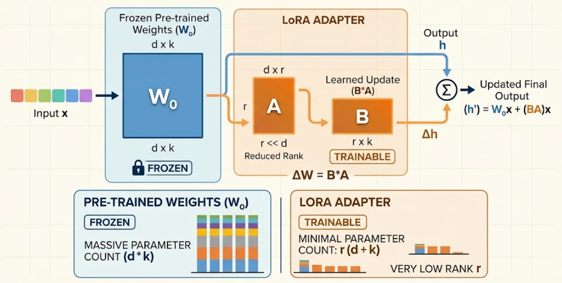
LoRA observes that the useful parameter change for a downstream task—like adapting a general model to parse complex SEC 10-K filings— often has a much lower intrinsic dimension than the original weight matrix.
For a frozen weight matrix , LoRA learns an update:
Instead of training a massive dense matrix, the update is factorized into two smaller matrices:
Where and are trainable, is the adapter rank, and controls the scale. By keeping smaller than and , trainable parameters drop drastically from to approximately .
For example, a square update contains 589,824 parameters. A rank-16 LoRA factorisation contains:
trainable parameters—24 times fewer for that matrix. The saving depends on the matrix shape, chosen rank, and number of modules adapted.
The low-rank hypothesis is not that the original weight matrix is low rank. It is that the task-specific change can often be expressed through a much smaller number of useful directions. LoRA learns those directions while leaving frozen.
LoRA is commonly applied to attention projection layers and sometimes to the feed-forward projections as well. A higher rank provides more adaptation capacity but increases memory, storage, and the risk of fitting noise. Rank is therefore a model-selection parameter, not a quality setting that should always be maximised.
Initialization, Scaling, and Target Modules
LoRA must begin without disturbing the pretrained model. A common initialization gives one factor non-zero random values and initializes the other to zero. The standard Hugging Face PEFT initialization sets with random values and to zero. Because , the first forward pass behaves exactly like the base model.
Rank () dictates the adapter's learning capacity and parameter count, while the ratio scales the update. There is no universally optimal ratio, so both parameters require empirical tuning for your specific dataset.
While early LoRA research focused strictly on attention projections, modern LLM recipes often target a wider array of layers, including query, key, value, and output projections, as well as the gate, up, and down projections in the feed-forward network.
For our 10-K case study, setting target_modules="all-linear" ensures we target both attention and feed-forward projections without needing to hard-code model-specific layer names.
After training, you must decide how to deploy the LoRA update:
- Dynamic Swapping (Keep Separate): Highly memory-efficient if one base model serves several different tasks (e.g., swapping between a 10-K risk adapter and a general summarization adapter on the fly).
- Weight Merging (Fuse to Base): Merging the adapter into the base weights removes the separate adapter computation during inference. This is ideal when deploying a single, fixed variant dedicated purely to financial analysis.
The original method is detailed in LoRA: Low-Rank Adaptation of Large Language Models. The current PEFT implementation exposes rank, scaling, dropout, and target
modules through LoraConfig (see the Hugging Face PEFT LoRA guide)
QLoRA: Reducing the Frozen Model's Memory
While LoRA reduces trainable parameters, the massive frozen base model must still be loaded into VRAM. QLoRA bridges this gap, making single-accelerator fine-tuning practical by loading the base model in 4-bit precision while training higher-precision LoRA adapters through the quantised model.
The vital distinctions are:
- Pretrained base weights are quantized to 4-bit and remain frozen.
- The LoRA adapter parameters remain trainable.
- Matrix multiplication computations occur in higher precision (e.g., BF16).
Core Mechanisms
QLoRA can make single-accelerator experiments practical, but it is not free. Quantisation introduces representation error, backend compatibility matters, and the final model must still be evaluated on the target task. The Transformers documentation recommends NF4 for training 4-bit base models.
QLoRA achieves these extreme memory savings through three specific innovations:
- Normal Float 4-bit (NF4): A 4-bit data type mathematically optimized to match the normal distribution of pretrained neural network weights. More values near 0, and fewer values at extremes.
- Double quantisation: Quantizing the scale constants used by the first quantisation step, further reducing metadata overhead.
- Paged optimisers: Leveraging unified memory paging to absorb temporary optimizer memory spikes-automatically pages optimizer states to CPU RAM when GPU runs out, preventing out-of-memory crashes.
The original QLoRA paper demonstrated fine-tuning a 65-billion-parameter model on a single 48 GB GPU. That result demonstrates the method's potential, not a universal hardware guarantee. Total training memory also includes quantisation metadata, activations, LoRA parameters, optimiser state, temporary workspaces, and a workload-dependent context length; it cannot be inferred from the raw 4-bit weight size alone.
See:
QLoRA: Efficient Finetuning of Quantized LLMs
Hugging Face bitsandbytes guide
Part III: Evaluating a Fine-Tuned Model
Evaluation asks a much broader question than whether training loss decreased: did the adaptation produce a reliable, practical improvement on unseen data? Answering this requires rigorous baselines, protected test sets, task-level metrics, and error analysis.
Establishing Meaningful Baselines
Before declaring the fine-tuning a success, at minimum, compare the fine-tuned model with the unchanged model using the same test examples and decoding settings. The unchanged model should receive a strong prompt containing the task definition, output format, and, where appropriate, a small number of demonstrations.
A useful comparison can include:
- The base model with a zero-shot prompt.
- The base model with the strongest few-shot prompt.
- The fine-tuned model with its intended inference prompt.
This isolation proves whether your costly training process actually generated new capabilities, or if the same result could have been achieved through clever prompting alone.
Preventing Data Leakage
Training, validation, and test data have different purposes. Training examples produce parameter updates, validation examples guide model and hyperparameter selection, and the test set provides the final estimate after those decisions have been made.
A random train/test split is dangerous when documents contain duplicates, revisions, or repeated templates. Split by the unit that could leak—for example, document, customer, company, or time period—and keep near-duplicates in the same split. The test set should also represent the conditions under which the model will be used, including difficult and negative examples.
If you split your dataset randomly by paragraph, your test set will contain near-duplicates of your training data.
- Split by Entity: Group your splits by company ticker or CIK. This ensures the model is evaluated on entirely unseen organizations.
- Preserve Distributions: Ensure your test set represents the actual production environment, including difficult edge cases and negative examples (documents where no material risks are present).
Measuring the Application Contract
Perplexity and validation loss measure token prediction; it does not measure if the application works safely. Evaluation metrics should reflect the behaviour that users depend on:
| Evaluation Dimension | Example Measures |
|---|---|
| Task Accuracy | Precision, recall, F1, exact match, or field-level accuracy |
| Output Contract | Parse rate, schema validity, and allowed-value compliance |
| Grounding | Evidence validity, factual consistency, and unsupported-claim rate |
| Abstention | Accuracy when evidence is missing, irrelevant, or ambiguous |
| Robustness | Performance by input length, domain, difficulty, and unseen source |
| General capability | Regression tests for instruction following and unrelated tasks |
| Operational efficiency | Latency, throughput, memory use, and adapter storage |
Not every task needs every metric. A classifier may be judged primarily by precision, recall, and calibration; a structured extraction system also needs schema and evidence checks; an open-ended assistant requires a carefully defined human-review rubric.
Deterministic checks (like JSON parsing and exact-string matching for evidence) should be fully automated. However, semantic properties—such as completeness, faithfulness, clarity, and appropriate uncertainty often require a carefully defined human-review rubric or a validated LLM-as-a-judge pipeline.
Human comparisons should use a written rubric and anonymised outputs so that reviewers do not know which system produced each response. Report results by important slices rather than only as one average, and inspect representative false positives, false negatives, hallucinations, and formatting failures.
Ultimately, a fine-tuned model is successful only when its improvement over the baseline justifies its training, evaluation, storage, and serving costs.
Part IV: Hands-On SEC 10-K Risk-Analysis Case
The analysis notebooks can be found here.
1. Problem statement, objectives, and task
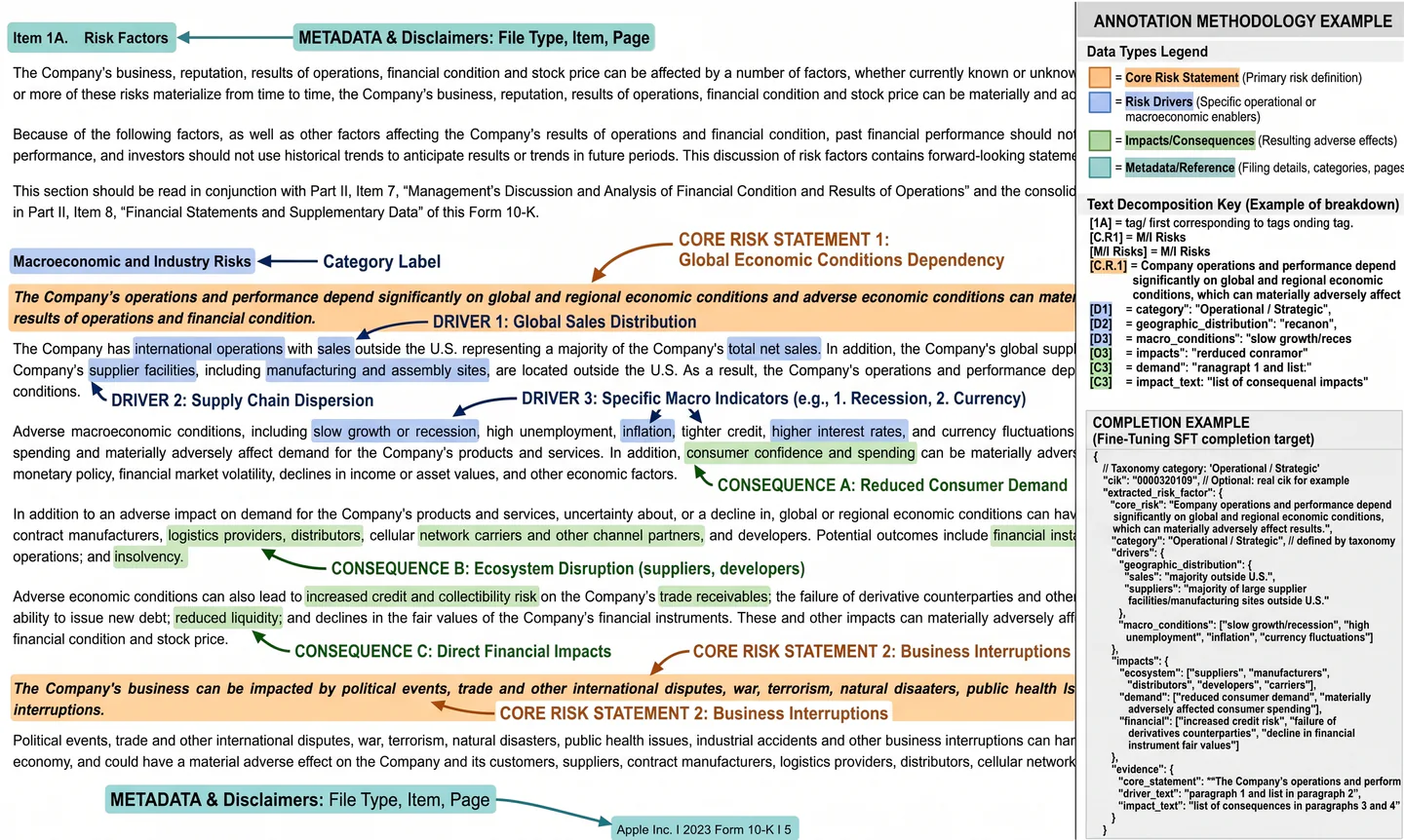
Risk disclosures in Item 1A of a 10-K are valuable to analysts, compliance teams, and risk managers, but they are lengthy, repetitive, and expressed in unstructured language. Similar risks can be described differently across companies, while manual categorisation and summarisation may be inconsistent.
The proposed system is an analytical assistant rather than an investment or materiality engine. It converts a supplied disclosure passage into a structured, reviewable record. Its objectives are to:
- reduce the effort needed to identify disclosed risks;
- normalise those risks into a consistent schema;
- preserve exact evidence for traceability; and
- determine whether fine-tuning improves on a well-prompted base model.
The model receives a 10-K excerpt:
A substantial portion of our cash is held outside our home market.
Restrictions on transferring those funds or adverse currency movements
could reduce the amount available for domestic operations.
and outputs:
{
  "risks": [
    {
      "category": "Financial",
      "summary": "Transfer restrictions and currency movements may reduce cash available for domestic operations.",
      "evidence": "Restrictions on transferring those funds or adverse currency movements could reduce the amount available for domestic operations."
    }
  ],
  "insufficient_evidence": false
}
It must identify zero or more risks, assign an experiment-specific category, summarise each risk, copy supporting evidence, and abstain when the passage does not support an extraction. It must not use outside facts or predict whether the risk will occur. Comparing disclosures between years is a possible downstream task, but it is deliberately excluded from this first experiment.
2. The data problem
The modelling task begins with a data-engineering problem. A production pipeline would retrieve filings from SEC EDGAR, identify Item 1A, remove filing markup, split the section into coherent disclosure passages, and retain enough provenance to trace every passage back to its source. At minimum, a record should preserve the company identifier, accession number, filing date, source URL, section, and source text.
This experiment uses synthetic disclosures so that the workflow is reproducible and redistributable. The synthetic data is suitable for testing the training and evaluation pipeline, but it cannot establish performance on real filings.
The source of truth is a canonical annotation record rather than a model-specific prompt. A simplified record looks like this:
{
  "example_id": "train_001",
  "split": "train",
  "issuer_id": "issuer_01",
  "filing_year": 2023,
  "source_text": "Restrictions on transferring those funds or adverse currency movements could reduce the amount available for domestic operations.",
  "risks": [
    {
      "category": "Financial",
      "summary": "Transfer restrictions and currency movements may reduce cash available for domestic operations.",
      "evidence": "Restrictions on transferring those funds or adverse currency movements could reduce the amount available for domestic operations."
    }
  ],
  "insufficient_evidence": false
}
The risk taxonomy is deliberately small and operational. It standardises the expected output without pretending to be a universal classification of 10-K risks:
| Category | Examples of disclosed risk |
|---|---|
| Financial | Liquidity, credit, currency, interest-rate, or funding exposure |
| Operational | Supply-chain, manufacturing, capacity, or business-continuity disruption |
| Market | Demand, pricing, competition, or macroeconomic exposure |
| Regulatory | Laws, investigations, compliance obligations, or policy changes |
| Cybersecurity | Security incidents, system compromise, or data exposure |
| Strategic | Acquisitions, concentration, execution, or business-model risk |
| People | Talent retention, labour availability, leadership, or workforce risk |
The dataset contains 68 examples:
| Split | Examples | Design |
|---|---|---|
| Training | 40 | 2022–2023 disclosures from development issuers |
| Validation | 12 | 2024 disclosures from the same issuers |
| Test | 16 | 2025 disclosures from entirely held-out issuers |
All splits contain positive, negative, and multi-risk examples. Negative examples teach abstention; multi-risk examples prevent the model from assuming that every passage contains exactly one label. Evidence must be copied exactly from the source text, which makes grounding mechanically verifiable.
The split is designed to reduce leakage. Development issuers appear only in the training and validation sets, while test issuers are held out completely. Normalised passages are also compared across splits so that near-duplicate language cannot turn evaluation into memorisation.
Only after these checks is each canonical record converted into the conversational prompt-completion structure required for SFT:
{
  "prompt": [
    {"role": "system", "content": "Extract only risks supported by the supplied 10-K excerpt..."},
    {"role": "user", "content": "<10-K excerpt>"}
  ],
  "completion": [
    {"role": "assistant", "content": "{\"risks\": [...], \"insufficient_evidence\": false}"}
  ]
}
Keeping canonical annotations separate from rendered prompts makes it possible to change a chat template or model family without rewriting the labels. Before training, the pipeline validates the schema, category values, exact evidence spans, abstention logic, split membership, near-duplicate controls, and token lengths.
3. Methodology: a controlled LoRA–QLoRA comparison
The experiment starts from Qwen/Qwen3-0.6B. It is an instruction-following
causal language model small enough for an accessible demonstration while still
supporting the chat-template and structured-generation workflow used by larger
models. Starting from an instruction model is intentional: the experiment is
specialising an existing assistant for a constrained extraction behaviour, not
trying to teach a base model how to follow instructions from a small dataset.
Two adapters are trained against the same checkpoint and data. The ordinary LoRA run keeps the frozen base weights in BF16 or FP16. The QLoRA run stores those frozen weights in four-bit NF4 and performs adapter computation at a higher precision. In both cases, the trainable update is LoRA.
| Setting | Value |
|---|---|
| Task | Grounded multi-risk extraction to JSON |
| Base checkpoint | Qwen/Qwen3-0.6B |
| Training objective | Completion-only causal language modelling |
| LoRA rank and alpha | r=16, alpha=32 |
| Target modules | All linear attention and feed-forward projections |
| Context limit | 1,024 tokens |
| Evaluation systems | Base zero-shot, base few-shot, LoRA, and QLoRA |
The intended experimental difference is therefore how the frozen base model is stored during training:
| Training arm | Frozen base model | Trainable parameters |
|---|---|---|
| LoRA | BF16 or FP16 | LoRA adapter |
| QLoRA | Four-bit NF4 with double quantisation | LoRA adapter |
To make the comparison meaningful, both arms use the same dataset splits, prompt format, maximum sequence length, rank, scaling, target modules, optimiser settings, random seed, and evaluation protocol. The LoRA configuration is:
lora_config = LoraConfig(
    task_type="CAUSAL_LM", # The model performs causal next-token generation
    r=16,                  # Capacity and size of the low-rank update
    lora_alpha=32,         # Scale applied to that update
    lora_dropout=0.05,     # Regularisation
    target_modules="all-linear", # Model layers receiving LoRA adapters, generally including: attention and feed-forward network
    bias="none",           # Whether existing bias parameters are trained
)
target_modules="all-linear" applies adapters to the model's linear attention
and feed-forward projections. It is convenient for this experiment because it
avoids hard-coding architecture-specific module names, although a production
study should still inspect the matched modules and report them.
This is not a comparison between two different adapter algorithms. QLoRA still trains LoRA parameters; quantisation reduces the memory required to keep the frozen base model available during training. The expected trade-off is lower peak memory, potentially accompanied by a small change in training dynamics.
The controlled question is therefore whether QLoRA reduces peak training memory without materially reducing extraction accuracy, grounding, or schema compliance relative to ordinary LoRA.
4. Training with completion-only SFT
Each training arm uses the same prepared prompt-completion records and LoRA
configuration. The experiment is controlled by a TRAINING_METHOD flag; only the frozen base-model loading path changes.
For QLoRA, we dynamically inject a 4-bit quantization configuration:
if TRAINING_METHOD == "qlora":
    load_kwargs["quantization_config"] = BitsAndBytesConfig(
        load_in_4bit=True,
        bnb_4bit_quant_type="nf4",
        bnb_4bit_use_double_quant=True,
        bnb_4bit_compute_dtype=compute_dtype,
    )
Configuring the Trainer
The tutorial configuration uses five epochs, a learning rate of 2e-4, an adapter rank of 16, and memory-saving techniques like gradient accumulation and checkpointing.
A maximum sequence length of 1024 accommodates the SEC excerpts. These are experiment settings rather than universal defaults.
The trainer receives the conversational records and is explicitly instructed to use completion-only loss:
training_args = SFTConfig(
    learning_rate=2e-4,
    num_train_epochs=5,
    per_device_train_batch_size=1,
    gradient_accumulation_steps=4,
    gradient_checkpointing=True,
    max_length=1024,
    completion_only_loss=True,
    eval_strategy="epoch",
    save_strategy="epoch",
)

trainer = SFTTrainer(
    model=model,
    args=training_args,
    processing_class=tokenizer,
    train_dataset=dataset["train"],
    eval_dataset=dataset["validation"],
)
Passing processing_class=tokenizer is critical: it tells the trainer how to apply the chat template, render the strings, and convert them into token IDs.
Understanding the Training Batch Tensors
Behind the scenes, trainer.get_train_dataloader() constructs the batches that enter the model. Each batch is composed of three aligned integer matrices,
typically with the shape [batch_size, sequence_length].
| Tensor | Purpose |
|---|---|
input_ids | Vocabulary index integers representing the rendered system message, user excerpt, and assistant completion. |
attention_mask | Contains 1 for real tokens and 0 for padding, telling the attention mechanism which positions to ignore.e |
labels | The target tokens used for gradient calculation. Prompt and padding positions are set to -100. |
Here is a conceptual look at a single training row showing how completion-only loss masks the prompt:
| Position | Content | input_ids | attention_mask | labels (Target) |
|---|---|---|---|---|
| 0 | System | 101 | 1 | -100 (Ignored) |
| 1 | User | 205 | 1 | -100 (Ignored) |
| 2 | User | 301 | 1 | -100 (Ignored) |
| 3 | Assistant | 401 | 1 | 401 (Supervised) |
| 4 | Assistant | 402 | 1 | 402 (Supervised) |
| 5 | Padding | 0 | 0 | -100 (Ignored) |
While the visual representation above is simplified, understanding the mechanics of these tensors is essential for debugging:
-
The Causal Shift: Notice that at supervised positions (3 and 4), the labels ID is identical to the input_ids value. This is because PyTorch's causal language modeling loss internally shifts the labels by one position. The model's prediction at position is evaluated against the label at position .
-
Dynamic Padding: With
per_device_train_batch_size=1, each matrix has exactly one row. If the batch size increases, shorter examples are dynamically padded to match the longest sequence in that specific batch. The sequence length is capped at 1,024, but most batches will be narrower than that. -
Indices vs. Embeddings: The
input_idsmatrix does not contain dense vector embeddings. It contains simple vocabulary indices that the model uses to look up the actual embeddings, which then produce a hidden-state tensor of shape[batch_size, sequence_length, d_model].
Finally, each run records the model identifier, random seed, LoRA settings, trainable parameters, peak GPU memory, and training duration. While validation loss is logged to monitor optimization health, it does not replace the rigorous task-level evaluation detailed in Part III.
Each run records the model identifier, random seed, LoRA settings, library versions, trainable and total parameters, training duration, peak GPU memory, and trainer metrics. Validation loss monitors optimisation; it does not replace task-level evaluation.
5. Evaluation and base-model comparison
The evaluation protocol is designed to compare four systems under the same held-out data, output limit, and deterministic decoding policy:
- the unchanged base model with a zero-shot instruction;
- the unchanged base model with representative positive and negative examples;
- the LoRA adapter; and
- the QLoRA adapter.
The completed run used Qwen/Qwen3-0.6B and all 16 held-out synthetic examples from eight issuers. Inference ran in FP16 on Apple MPS.
Both adapters were loaded separately onto the same higher-precision base checkpoint used by the baselines.
The comparison therefore measures the behaviour learned by each adapter rather than comparing FP16 and 4-bit inference.
| Metric | What it tests |
|---|---|
| JSON and schema validity | Whether downstream code can safely consume the response. |
| Risk precision, recall, and F1 | Whether labelled risks are extracted without extras or omissions. |
| Category macro F1 | Whether performance extends beyond the most frequent category. |
| Evidence validity | Whether each quoted span explicitly occurs in the supplied excerpt. |
| Unsupported-evidence rate | How often generated evidence is hallucinated. |
| Abstention accuracy | Whether non-risk passages are rejected correctly. |
| Latency and tokens per second | Runtime cost under the declared test setup. |
| Peak training memory and duration | Training-resource footprint (comparable only on identical hardware). |
| Adapter size | Per-task storage requirement. |
Note: Invalid JSON, unsupported evidence, and missed risks are explicitly decoupled. A schema failure is a formatting error, not automatically a hallucinated claim. The automated metrics below precede our blinded human-review rubric for summary faithfulness.
Quality Results
| System | JSON valid | Schema valid | Risk precision | Risk recall | Risk F1 | Category macro F1 | Evidence valid | Abstention accuracy |
|---|---|---|---|---|---|---|---|---|
| Base, zero-shot | 100.0% | 56.3% | 11.1% | 6.7% | 8.3% | 2.4% | 100.0% | 43.8% |
| Base, few-shot | 100.0% | 100.0% | 33.3% | 20.0% | 25.0% | 20.0% | 100.0% | 81.3% |
| LoRA adapter | 100.0% | 100.0% | 63.6% | 46.7% | 53.8% | 76.2% | 100.0% | 100.0% |
| QLoRA adapter | 100.0% | 100.0% | 58.3% | 46.7% | 51.9% | 70.1% | 91.7% | 93.8% |
Few-shot prompting was already a much stronger baseline than the zero-shot instruction. Relative to that stronger baseline, Both adapters maintained perfect schema validity. LoRA significantly outperformed the strong few-shot baseline, boosting risk F1 by 28.8 points and abstention accuracy by 18.8 points. QLoRA followed closely. While LoRA retained a slight edge in precision and grounding over QLoRA, the small sample size () means these figures serve to demonstrate our pipeline's analytical rigor rather than proving general algorithmic superiority.
Efficiency Results
| System | Mean latency | Output tokens/s | Adapter size | Peak training memory | Training time |
|---|---|---|---|---|---|
| Base, zero-shot | 1.47 s | 58.90 | — | — | — |
| Base, few-shot | 0.72 s | 54.30 | — | — | — |
| LoRA adapter | 1.19 s | 36.67 | 49.46 MiB | Not recorded | 63.63 s |
| QLoRA adapter | 1.25 s | 36.41 | 49.46 MiB | 1.63 GiB | 84.84 s |
Latency was measured sequentially on Apple MPS and includes varying output lengths and unmerged PEFT overhead. Consequently, these figures serve as an observational baseline rather than a hardware-independent benchmark. Both adapters predictably share an identical 49.46 MiB footprint; 4-bit quantization compresses the frozen base model during training, but does not alter the saved adapter's dimensions.
Similarly, the training times (63.63s for LoRA; 84.84s for QLoRA) and memory allocations (a 1.27 GiB end-of-run snapshot for LoRA versus a 1.63 GiB recorded peak for QLoRA) strictly reflect this specific MPS environment. Because the memory profiling captured different lifecycle phases, these values do not provide a controlled baseline for quantifying QLoRA's memory savings.
The Path to Production
Aggregate metrics only tell part of the story. Meaningful evaluation requires slicing errors across sectors, risk categories, negative examples, and multi-risk passages. While our 16-example synthetic dataset successfully validates the evaluation mechanics, proving true production readiness demands significantly more rigor, including:
- An expansive, strictly held-out test set of manually reviewed EDGAR excerpts.
- Systematic uncertainty estimation and blinded domain review.
- Broad regression testing outside the core extraction task.
Ultimately, fine-tuning earns its place in the stack only if an adapter demonstrably outperforms the strongest reasonable prompting baseline, flawlessly preserves evidence grounding, and delivers a performance gain that explicitly justifies the added operational complexity.
微調(fine-tuning)的目的,是讓預訓練模型更穩定地執行特定任務或呈現特定行為。真正困難的往往不是啟動訓練,而是明確定義目標行為、建立一致且具代表性的範例,並證明訓練後的 adapter 確實優於經過良好提示設計的基準模型。
本文分為四個部分:
閱讀本文前,建議先熟悉純解碼器 Transformer 的基本原理,可參考 LLM 預訓練:深入解析純解碼器 Transformer 作為背景知識。
第一部分:微調總覽
當目標行為會反覆出現、可以清楚定義,而且只靠提示詞(prompting)仍難以穩定達成時,才適合考慮微調。微調是模型適應方法之一,通常不應作為預設的第一步。
微調是正確的工具嗎?
在投入運算資源與時間前,應先以少樣本提示(few-shot prompting)或 檢索增強生成(RAG) 建立具競爭力的基準。 提示詞與 RAG 適合在執行時提供指令、事實與上下文;微調則較適合調整模型反覆執行任務時的行為、格式與領域適應方式。
在以下情況,你可以考慮從提示詞轉向微調:
- 上下文視窗(context window)經常被複雜且高度特定的少樣本範例占滿。
- 模型必須以高遵循率產生固定格式(例如符合指定 JSON schema 的 10-K 風險紀錄),而只靠提示詞仍不夠穩定。
- 成本或延遲限制要求使用較小、經任務適應的開放權重模型,取代規模較大的專有模型。
| 需求 | 建議做法 |
|---|---|
| 改善單次的指令表現 | 提示工程(Prompt engineering) |
| 存取即時或私有文件 | 檢索增強生成(RAG) |
| 加入頻繁變動的財務事實 | 檢索增強生成(RAG),而非仰賴模型記憶 |
| 重現穩定的語氣、分類體系或輸出格式 | 微調 |
| 從標註範例中學習一致的判斷 | 微調 |
這些做法可以互補。在 10-K 應用中,檢索負責提供相關 SEC 揭露內容,微調則讓模型更一致地擷取、分類並格式化資訊。
監督式微調(SFT)的訓練目標
模型適應可以採用多種訓練目標。例如,模型可能先透過持續預訓練(continued pretraining)接觸領域語言,再以 SFT 學習任務行為,最後使用 DPO 等偏好調整方法,或以 RLHF 等強化學習方法進一步對齊輸出。
因此,「微調」不是單一訓練目標,而是包含多種模型適應方法的概括用語。
| 方法 | 學到的內容 |
|---|---|
| 持續預訓練 | 透過下一個 token 預測,學習領域語言、術語與文件模式 |
| 監督式微調(SFT) | 從標註範例中學習期望的輸入到輸出行為 |
| 偏好調整 | 學習兩個回應中哪一個較好,常用方法如直接偏好最佳化(DPO) |
| 強化學習 | 學習能最大化獎勵訊號的行為,常用方法如 RLHF 或 RLAIF |
本次 10-K 實驗採用 SFT,因為期望的輸入與輸出可以表示為已標註的 prompt-completion 配對。
因果語言建模(causal language modeling)這個目標本身,和預訓練階段相比並沒有根本上的改變:模型依然是在預測下一個 token。真正改變的是資料的分布。原始文件教會模型的只是「接續文字」,而經過整理的 SFT 示範範例,則教會模型以一致、結構化的方式回應特定類型的請求。
聊天樣板(Chat Template):訓練的契約
一段以 role 與 content 物件表示的對話,最終都必須被轉換成一串 token 序列。聊天樣板(chat template)的作用,就是插入用來標記 system、user、assistant 以及訊息邊界的控制符號(control token):
結構化訊息
        ↓ 模型專屬的聊天樣板
[system 控制符號]     指令
[user 控制符號]       請求
[assistant 控制符號]  回應
        ↓ 分詞器(tokenizer)
訓練用的 Token ID
不同模型家族使用不同的控制符號。例如,Llama 3 使用 <|start_header_id|> 與 <|eot_id|> 組織對話,Mistral 則使用 [INST] 與 [/INST]。訓練與推論都應使用與 tokenizer 及模型相符的聊天樣板;套用其他模型的格式,可能降低輸出品質。
transformers 函式庫透過 tokenizer.apply_chat_template 這個方法,將這個轉換過程開放給使用者:
from transformers import AutoTokenizer

tokenizer = AutoTokenizer.from_pretrained("mistralai/Mistral-7B-Instruct-v0.1")
chat = [
  {"role": "system", "content": "You are a financial assistant."},
  {"role": "user", "content": "Analyze this 10-K excerpt."},
  {"role": "assistant", "content": "{\"risks\": [...]}"}
]

# 這會輸出一個帶有控制符號、格式正確的扁平字串
tokenizer.apply_chat_template(chat, tokenize=False)
Hugging Face chat-template guide
損失遮罩(Loss Masking):只計算回應部分的損失
完成格式化後,還要決定哪些 token 會計入訓練損失。在 completion-only 訓練中,prompt token 提供必要上下文,但不納入損失;模型只根據 assistant 回應部分的預測誤差更新參數。
我們透過標籤遮罩(label mask)來達成這件事。忽略值 -100 會告訴 PyTorch 的交叉熵(cross-entropy)實作,不要對這些位置計分:
Token:  [系統指令]     [使用者提示]     [助理回應]
標籤:   [   -100   ]   [   -100   ]     [ 在此計算損失 ]
將 prompt 對應的 label 設為忽略值後,學習訊號就會集中在模型需要產生的回應上。在目前版本的 TRL(Transformer Reinforcement Learning)中,prompt-completion 格式的資料集預設採用 completion-only 損失;對話格式資料集則可以設定 assistant_only_loss=True,前提是聊天樣板能提供有效的 generation mask。
(實作細節請參考 TRL SFTTrainer loss-masking documentation)
在某些情境下,對完整序列計算損失同樣合理。因此,是否只監督回應部分,應根據資料格式與訓練目標明確決定,而不是視為通用規則。
全參數微調 vs. PEFT
全參數微調(full fine-tuning)會更新模型中的所有參數,因此需要大量記憶體存放梯度與最佳化器狀態。每個任務版本通常也要保存一份完整模型權重。
參數高效微調(Parameter-Efficient Fine-Tuning,PEFT)則凍結大部分基礎模型,只訓練少量新增或選定的參數。一種常見分類方式,將 PEFT 概括為三類策略:
| PEFT 策略 | 運作機制 | 代表方法 |
|---|---|---|
| 加法式(Additive) | 凍結基礎模型,並加入新的可訓練參數。 | Adapter 模組、prompt tuning、prefix tuning、P-tuning |
| 選擇式(Selective) | 只更新既有參數中,經過挑選的一小部分。 | BitFit、LayerNorm tuning、部分層解凍 |
| 重參數化(Reparameterisation) | 用一個精簡的數學結構,來表達權重的更新。 | LoRA、AdaLoRA、DoRA |
LoRA 屬於重參數化方法;QLoRA 則是在量化後、保持凍結的基礎模型上訓練 LoRA adapter。PEFT 可以降低訓練與儲存成本,卻無法彌補資料與標註品質不足的問題。
這套分類方式,出自 Scaling Down to Scale Up: A Guide to Parameter-Efficient Fine-Tuning。
第二部分:LoRA 與 QLoRA
LoRA:低秩適應(Low-Rank Adaptation)
LoRA 的核心假設是:針對特定下游任務所需的權重更新,其內在維度(intrinsic dimension)可能遠低於原始權重矩陣。換句話說,即使原始矩陣很大,有效的任務調整也可能只需要少數方向。
對於一個凍結的權重矩陣 ,LoRA 學習的是一個更新量:
它不直接訓練一個龐大的密集矩陣,而是把這個更新量,分解成兩個較小的矩陣:
其中 與 是可訓練的參數, 是 adapter 的秩(rank),而 則控制更新量的縮放比例。只要讓 遠小於 與 ,可訓練參數量就能從 大幅降低到約 。
舉例來說,一個 的方陣更新量,包含 589,824 個參數。而一個 rank-16 的 LoRA 分解,則只包含:
個可訓練參數,約為完整矩陣更新量的 1/24。實際節省幅度取決於矩陣形狀、rank,以及套用 adapter 的模組數量。
低秩假設(low-rank hypothesis)不是指原始權重矩陣本身為低秩,而是任務特定的更新量 可以由較少的方向近似表示。LoRA 學習這些方向,同時維持 凍結。
LoRA 通常套用在注意力機制(attention)的投影層上,有時也會套用到前饋網路(feed-forward)的投影層。較高的 rank 能提供更多的適應能力,但也會增加記憶體用量、儲存空間,以及擬合雜訊的風險。因此 rank 是一個需要透過模型選擇來決定的參數,而不是一個「越高越好」的品質設定。
初始化、縮放與 Target Modules
LoRA 通常會初始化為不改變基礎模型輸出的狀態。Hugging Face PEFT 的標準做法,是將 設為隨機值、 初始化為零。此時 ,因此訓練開始前的前向傳播(forward pass)與基礎模型一致。
Rank()決定 adapter 的容量與參數量, 則控制更新量的縮放幅度。兩者沒有適用所有資料集的單一最佳設定,應透過驗證實驗選擇。
原始 LoRA 研究主要針對注意力投影層;現代 LLM 訓練配方則常涵蓋更廣的線性層,包括 Query、Key、Value、Output 投影,以及前饋網路中的 gate、up、down 投影。本次 10-K 案例使用 target_modules="all-linear",避免針對特定模型手動列出模組名稱;實際匹配範圍仍應在訓練前確認。
訓練完成後,你還必須決定如何部署這個 LoRA 更新量:
- 動態載入(保持分離):同一個基礎模型可以搭配多個任務 adapter,例如在「10-K 風險分析」與「一般摘要」之間切換。這有利於版本管理與重複使用基礎權重。
- 權重合併:將 adapter 更新合併回基礎權重,可以省去推論時額外套用 adapter 的運算,適合部署單一固定版本;代價是失去快速切換 adapter 的彈性。
原始方法的詳細內容,可參考 LoRA: Low-Rank Adaptation of Large Language Models。目前的 PEFT 實作,則透過 LoraConfig 開放 rank、縮放比例、dropout 與 target modules 等設定(詳見 Hugging Face PEFT LoRA guide)。
QLoRA:降低凍結模型的記憶體用量
LoRA 雖然減少了可訓練參數,凍結的基礎模型仍須載入裝置記憶體。QLoRA 進一步以 4-bit 格式載入基礎權重,並以較高精度進行運算及訓練 LoRA adapter,藉此降低訓練期間的記憶體需求。
幾個關鍵的區別在於:
- 預訓練的基礎權重被量化為 4-bit,並維持凍結狀態。
- LoRA adapter 的參數仍然是可訓練的。
- 矩陣乘法運算,則是以較高精度進行(例如 BF16)。
核心機制
QLoRA 可以讓部分原本無法在單一加速器執行的實驗成為可能,但量化會引入近似誤差,且支援程度取決於硬體與軟體後端。最終模型仍須在目標任務上評估。Transformers 文件建議,訓練 4-bit 基礎模型時使用 NF4。
QLoRA 之所以能達到如此極端的記憶體節省,靠的是三項具體的創新:
- Normal Float 4-bit(NF4): 一種針對常態分布權重設計的 4-bit 資料型別,在有限的表示值中更有效地配置常見權重範圍。
- 雙重量化(Double quantisation): 再次量化第一次量化所使用的縮放常數,降低中繼資料的額外空間。
- 分頁最佳化器(Paged optimisers): 利用統一記憶體分頁(unified memory paging)處理最佳化器狀態的暫時性記憶體峰值,降低 GPU 記憶體不足的風險。
QLoRA 原始論文展示了在單張 48 GB GPU 上微調 650 億參數模型的結果,但這不代表所有模型與設定都有相同硬體需求。總記憶體還包含量化中繼資料、激活值、LoRA 參數、最佳化器狀態、暫存工作空間,以及受上下文長度影響的張量,不能只根據 4-bit 權重大小推算。
見:
QLoRA: Efficient Finetuning of Quantized LLMs
Hugging Face bitsandbytes guide
第三部分:評估微調後的模型
評估要回答的不只是「訓練損失是否下降」,而是模型在未見資料上,是否產生可靠且具實務意義的改善。這需要具競爭力的基準、與開發流程隔離的測試集、任務層級指標及錯誤分析。
建立有意義的基準模型
在判定微調成功前,至少應使用相同的測試資料與解碼設定,比較微調模型和未修改的基礎模型。基礎模型應搭配完善的提示詞,明確說明任務與輸出格式,必要時加入少量示範範例。
一個有用的比較,可以包含:
- 使用 zero-shot 提示詞的基礎模型。
- 使用最強 few-shot 提示詞的基礎模型。
- 使用其預期推論提示詞的微調後模型。
這樣的比較可以判斷,訓練帶來的改善是否超過提示詞設計本身所能達到的效果。
防止資料外洩
訓練集、驗證集與測試集具有不同用途:訓練集用於更新參數,驗證集用於選擇模型與超參數,測試集則應在所有開發決策完成後,提供最終的泛化表現估計。
若文件包含重複內容、修訂版本或固定樣板,隨機切分很容易造成資料外洩。資料應依可能產生關聯的單位切分,例如文件、客戶、公司或時間區間,並確保近似重複(near-duplicate)內容位於同一資料分割。測試集也應反映實際使用情境,包括困難案例與負面案例。
如果你依段落隨機切分資料集,測試集中就會出現與訓練資料高度相似的內容。
- 依實體切分:依公司股票代號或 CIK 來分組。這能確保模型是在完全沒見過的公司上接受評估。
- 維持代表性:確保測試集能反映實際正式環境,包括困難的邊界案例,以及不包含可擷取風險的負面案例。
衡量應用程式的契約
困惑度(perplexity)與驗證損失衡量 token 預測表現,卻無法完整反映應用程式是否可靠。評估指標應直接對應使用者與下游系統所依賴的行為:
| 評估面向 | 範例指標 |
|---|---|
| 任務準確度 | 精確率(Precision)、召回率(Recall)、F1、完全匹配(exact match),或欄位層級的準確度 |
| 輸出契約 | 解析成功率、schema 有效性,以及允許值的合規性 |
| 依據性(Grounding) | 證據有效性、事實一致性,以及缺乏依據的宣稱比例 |
| 拒答(Abstention) | 在證據缺失、不相關或含糊不清時的判斷準確度 |
| 穩健性 | 依輸入長度、領域、難度與未見過的來源而定的表現 |
| 一般能力 | 針對指令遵循能力與不相關任務的回歸測試 |
| 營運效率 | 延遲、吞吐量、記憶體用量,以及 adapter 儲存空間 |
並非每一項任務都需要用到所有指標。一個分類器,可能主要依精確率、召回率與校準程度來評判;一個結構化擷取系統,還需要 schema 與證據檢查;而一個開放式的助理,則需要一套經過仔細定義的人工審查準則(rubric)。
可明確判定的檢查,例如 JSON 解析與證據精確字串比對,應盡量自動化。完整性、忠實度、清晰度與適當的不確定性表達等語意品質,則通常需要明確的人工審查準則,或經過驗證的 LLM-as-a-judge 流程。
人工比較時,應該使用書面的審查準則,並將輸出結果匿名化,讓審查者無法得知每個回應是由哪個系統產生。結果的呈現方式,也應該依重要的切分維度分別報告,而不是只給一個整體平均值,同時也要檢視具代表性的偽陽性、偽陰性、幻覺內容,以及格式錯誤的案例。
最終,微調是否成功,取決於相對基準模型的改善幅度,能否合理抵銷訓練、評估、儲存、部署與維運成本。
第四部分:實作案例——SEC 10-K 風險分析
相關的分析 notebook 可參考 llm-fine-tuning-10K-report。
1. 問題定義、目標與任務
10-K 中 Item 1A 的風險揭露內容,對分析師、法遵團隊與風險管理人員而言相當有價值,但這些內容通常又長又重複,而且以非結構化的語言呈現。類似的風險,在不同公司之間可能會用完全不同的方式描述,而人工分類與摘要,也可能出現不一致的情況。
本案例將系統定位為分析輔助工具,而非投資建議或重大性(materiality)判斷系統。它會將風險揭露段落轉換為結構化、可供人工審查的紀錄,目標包括:
- 降低初步辨識與整理揭露風險所需的人力;
- 以一致的 schema 表示風險;
- 保留原文證據,維持可追溯性;以及
- 判斷微調模型是否優於具競爭力的提示基準。
模型收到的輸入,是一段 10-K 摘錄:
A substantial portion of our cash is held outside our home market.
Restrictions on transferring those funds or adverse currency movements
could reduce the amount available for domestic operations.
輸出則是:
{
  "risks": [
    {
      "category": "Financial",
      "summary": "Transfer restrictions and currency movements may reduce cash available for domestic operations.",
      "evidence": "Restrictions on transferring those funds or adverse currency movements could reduce the amount available for domestic operations."
    }
  ],
  "insufficient_evidence": false
}
模型必須辨識零個或多個風險、套用本實驗定義的分類、為每項風險撰寫摘要、逐字複製支持該判斷的證據,並在段落不足以支持任何結果時拒答(abstain)。模型不得使用段落以外的資訊,也不負責預測風險是否會發生。跨年度揭露差異比較可作為後續任務,但不在本次實驗範圍內。
2. 資料問題
這項建模工作首先是資料工程問題。正式環境的資料管線需要從 SEC EDGAR 取得文件、辨識 Item 1A、移除標記語法(markup)、切分出語意完整的揭露段落,並保留足夠的來源資訊,使每段文字都能追溯至原始申報文件。每筆紀錄至少應包含公司識別碼、accession number、申報日期、來源網址、章節與原始文字。
本實驗使用合成(synthetic)揭露內容,使工作流程可以重現並自由分享。這份資料適合驗證訓練與評估管線,但不能用來推論模型在真實 SEC 申報文件上的表現。
資料的單一事實來源(source of truth)是標準化標註紀錄,而不是針對特定模型設計的 prompt。簡化後的紀錄如下:
{
  "example_id": "train_001",
  "split": "train",
  "issuer_id": "issuer_01",
  "filing_year": 2023,
  "source_text": "Restrictions on transferring those funds or adverse currency movements could reduce the amount available for domestic operations.",
  "risks": [
    {
      "category": "Financial",
      "summary": "Transfer restrictions and currency movements may reduce cash available for domestic operations.",
      "evidence": "Restrictions on transferring those funds or adverse currency movements could reduce the amount available for domestic operations."
    }
  ],
  "insufficient_evidence": false
}
這套風險分類體系(taxonomy)刻意保持精簡且可操作,用於統一本實驗的輸出標籤;它並不是涵蓋所有 10-K 風險的通用分類標準。
| 分類 | 揭露風險範例 |
|---|---|
| Financial(財務) | 流動性、信用、匯率、利率或資金曝險 |
| Operational(營運) | 供應鏈、製造、產能或營運持續性中斷 |
| Market(市場) | 需求、定價、競爭或總體經濟曝險 |
| Regulatory(法規) | 法律、調查、合規義務或政策變動 |
| Cybersecurity(資安) | 資安事件、系統遭入侵或資料外洩 |
| Strategic(策略) | 併購、集中度、執行力或商業模式風險 |
| People(人才) | 人才留任、勞動力供給、領導層或勞動力風險 |
整個資料集包含 68 筆範例:
| 切分 | 範例數 | 設計方式 |
|---|---|---|
| 訓練集 | 40 | 來自開發用發行人(issuer)的 2022–2023 年揭露內容 |
| 驗證集 | 12 | 來自相同發行人的 2024 年揭露內容 |
| 測試集 | 16 | 來自完全未見過的發行人的 2025 年揭露內容 |
每個資料分割都包含正例、負例與多風險範例。負例用於訓練拒答行為;多風險範例則避免模型將每個段落固定視為單一標籤。由於證據必須逐字取自原文,系統可以自動驗證輸出是否具有文字依據。
這項切分設計旨在降低資料外洩風險。開發用發行人只出現在訓練集與驗證集,測試用發行人則完全排除於開發過程之外。系統也會跨資料分割比對正規化後的段落,避免近似重複內容使評估結果被模型記憶能力高估。
只有在通過這些檢查之後,每一筆標準化紀錄,才會被轉換成 SFT 所需的對話式 prompt-completion 結構:
{
  "prompt": [
    {"role": "system", "content": "Extract only risks supported by the supplied 10-K excerpt..."},
    {"role": "user", "content": "<10-K excerpt>"}
  ],
  "completion": [
    {"role": "assistant", "content": "{\"risks\": [...], \"insufficient_evidence\": false}"}
  ]
}
將標準化標註與實際渲染的 prompt 分開,可以在更換聊天樣板或模型家族時沿用既有標註。訓練前,資料管線會驗證 schema、分類值、證據範圍、拒答邏輯、資料分割歸屬、近似重複內容與 token 長度。
3. 實驗方法:LoRA 與 QLoRA 的受控比較
本實驗以 Qwen/Qwen3-0.6B 為起點。它是具備指令遵循能力的因果語言模型,規模適合教學實驗,也支援聊天樣板與結構化生成流程。選擇指令模型,是因為本實驗要將既有助理特化為受限制的資訊擷取系統,而不是用小型資料集從頭建立指令遵循能力。
| 設定 | 值 |
|---|---|
| 任務 | 有事實根據的多風險擷取,輸出為 JSON |
| 基礎 checkpoint | Qwen/Qwen3-0.6B |
| 訓練目標 | Completion-only 的因果語言建模 |
| LoRA rank 與 alpha | r=16、alpha=32 |
| Target modules | 所有線性的注意力與前饋網路投影層 |
| 上下文長度上限 | 1,024 tokens |
| 評估對象 | 基礎模型 zero-shot、基礎模型 few-shot、LoRA、QLoRA |
這項實驗主要比較訓練期間凍結基礎模型的儲存精度:
| 訓練分支 | 凍結的基礎模型 | 可訓練參數 |
|---|---|---|
| LoRA | BF16 或 FP16 | LoRA adapter |
| QLoRA | 4-bit NF4,搭配雙重量化 | LoRA adapter |
為了提高可比性,兩個分支採用相同的資料集分割、prompt 格式、最大序列長度、rank、縮放比例、target modules、最佳化器設定、隨機種子與評估流程。LoRA 設定如下:
lora_config = LoraConfig(
    task_type="CAUSAL_LM", # 模型執行的是因果式的下一個 token 生成
    r=16,                  # 低秩更新量的容量與大小
    lora_alpha=32,         # 套用在該更新量上的縮放係數
    lora_dropout=0.05,     # 正則化(regularisation)
    target_modules="all-linear", # 套用 LoRA adapter 的模型層,一般包含注意力機制與前饋網路
    bias="none",           # 是否訓練既有的 bias 參數
)
target_modules="all-linear" 會將 adapter 套用到模型中符合條件的線性層,通常涵蓋注意力與前饋網路投影。本實驗藉此避免手動列出特定架構的模組名稱;正式實驗仍應檢查並記錄實際匹配的模組。
這不是兩種不同 adapter 演算法的比較。QLoRA 訓練的仍是 LoRA 參數;量化所降低的是訓練期間載入凍結基礎模型所需的記憶體,並可能使訓練數值行為產生些微差異。
因此,這項實驗要回答的是:相較於一般 LoRA,QLoRA 能否在維持擷取準確度、證據依據性與 schema 合規性的同時,降低訓練記憶體需求。
4. 使用 Completion-Only SFT 進行訓練
兩個訓練分支使用相同的 prompt-completion 紀錄與 LoRA 設定,並由 TRAINING_METHOD 旗標控制。主要差異是凍結基礎模型的載入方式。
在 QLoRA 的情況下,我們會動態注入一組 4-bit 量化設定:
if TRAINING_METHOD == "qlora":
    load_kwargs["quantization_config"] = BitsAndBytesConfig(
        load_in_4bit=True,
        bnb_4bit_quant_type="nf4",
        bnb_4bit_use_double_quant=True,
        bnb_4bit_compute_dtype=compute_dtype,
    )
設定 Trainer
本實驗訓練 5 個 epoch,學習率為 2e-4、adapter rank 為 16,並採用梯度累積(gradient accumulation)與 gradient checkpointing 降低記憶體需求。最大序列長度設為 1024,以容納 SEC 摘錄。這些是本次實驗設定,不應視為適用所有任務的預設值。
Trainer 接收這些對話格式的紀錄,並被明確指示使用 completion-only 損失:
training_args = SFTConfig(
    learning_rate=2e-4,
    num_train_epochs=5,
    per_device_train_batch_size=1,
    gradient_accumulation_steps=4,
    gradient_checkpointing=True,
    max_length=1024,
    completion_only_loss=True,
    eval_strategy="epoch",
    save_strategy="epoch",
)

trainer = SFTTrainer(
    model=model,
    args=training_args,
    processing_class=tokenizer,
    train_dataset=dataset["train"],
    eval_dataset=dataset["validation"],
)
processing_class=tokenizer 讓 trainer 使用指定 tokenizer 套用聊天樣板、渲染文字並轉換為 token ID。
理解訓練批次中的 Tensor
trainer.get_train_dataloader() 會建立實際輸入模型的 batch。每個 batch 通常包含三個形狀為 [batch_size, sequence_length]、位置彼此對齊的整數矩陣。
| Tensor | 用途 |
|---|---|
input_ids | 代表渲染後的 system 訊息、user 摘錄與 assistant completion 的詞彙索引整數。 |
attention_mask | 有效 token 為 1,padding 為 0,用來標示哪些位置應參與注意力運算。 |
labels | 用於梯度計算的目標 token。prompt 與 padding 的位置,都會被設為 -100。 |
以下用概念性的方式,呈現單一筆訓練資料的樣貌,展示 completion-only 損失是如何遮罩 prompt 的:
| 位置 | 內容 | input_ids | attention_mask | labels(目標) |
|---|---|---|---|---|
| 0 | System | 101 | 1 | -100(忽略) |
| 1 | User | 205 | 1 | -100(忽略) |
| 2 | User | 301 | 1 | -100(忽略) |
| 3 | Assistant | 401 | 1 | 401(監督學習) |
| 4 | Assistant | 402 | 1 | 402(監督學習) |
| 5 | Padding | 0 | 0 | -100(忽略) |
雖然上述示意經過簡化,但理解這些 tensor 的關係,有助於檢查資料整理與損失遮罩是否正確:
-
因果位移(Causal Shift):在受監督的位置(3 與 4),
labels的 ID 與input_ids相同。因果語言模型在計算損失時會對 logits 與 labels 做一個位置的位移,使位置 的輸出用來預測位置 的 token。 -
動態 Padding:當
per_device_train_batch_size=1時,每個矩陣只有一列。提高 batch size 後,較短範例會被 padding 至該 batch 的最長序列。序列長度上限為 1,024,但多數 batch 的實際寬度可能低於上限。 -
索引與 Embedding 的差異:
input_ids儲存的是詞彙索引,不是密集 embedding。模型會以這些索引查詢嵌入表,再產生形狀為[batch_size, sequence_length, d_model]的 hidden-state tensor。
每次訓練都會記錄模型識別碼、隨機種子、LoRA 設定、函式庫版本、可訓練與總參數量、訓練時間、裝置記憶體指標及 trainer 輸出。驗證損失用於監控最佳化過程,不能取代任務層級評估。
5. 評估與基礎模型比較
評估流程在相同的保留測試資料、輸出長度上限與決定性(deterministic)解碼設定下,比較四個系統:
- 使用 zero-shot 指令的未修改基礎模型;
- 搭配具代表性正例與負例的未修改基礎模型;
- LoRA adapter;以及
- QLoRA adapter。
完整實驗使用 Qwen/Qwen3-0.6B,測試集包含來自八家發行人的 16 筆合成範例。推論在 Apple MPS 上以 FP16 執行,兩個 adapter 都載入相同的高精度基礎 checkpoint。因此,品質比較反映的是 adapter 學到的任務行為,而不是 FP16 與 4-bit 推論格式之間的差異。
| 指標 | 檢驗內容 |
|---|---|
| JSON 與 schema 有效性 | 下游程式是否能解析並驗證回應。 |
| 風險精確率、召回率與 F1 | 模型是否正確擷取風險,並控制誤報與漏報。 |
| 分類 Macro F1 | 表現是否不只侷限在出現頻率最高的分類上。 |
| 證據有效性 | 每一段被引用的內容,是否確實出現在提供的摘錄之中。 |
| 無依據證據比例 | 證據欄位未出現在輸入摘錄中的比例。 |
| 拒答準確度 | 不含風險的段落,是否被正確地拒答。 |
| 延遲與每秒 token 數 | 在既定測試環境下的執行成本。 |
| 訓練記憶體峰值與所需時間 | 訓練所耗費的資源(僅在相同硬體下才具可比性)。 |
| Adapter 大小 | 每個任務所需的儲存空間。 |
備註:無效 JSON、無依據證據與遺漏風險是不同錯誤類型。Schema 失敗代表格式不符,不必然等同於內容缺乏事實依據。下列自動化指標是盲測人工審查摘要忠實度之前的第一層檢查。
品質結果
| 系統 | JSON 有效 | Schema 有效 | 風險精確率 | 風險召回率 | 風險 F1 | 分類 Macro F1 | 證據有效 | 拒答準確度 |
|---|---|---|---|---|---|---|---|---|
| 基礎模型,zero-shot | 100.0% | 56.3% | 11.1% | 6.7% | 8.3% | 2.4% | 100.0% | 43.8% |
| 基礎模型,few-shot | 100.0% | 100.0% | 33.3% | 20.0% | 25.0% | 20.0% | 100.0% | 81.3% |
| LoRA adapter | 100.0% | 100.0% | 63.6% | 46.7% | 53.8% | 76.2% | 100.0% | 100.0% |
| QLoRA adapter | 100.0% | 100.0% | 58.3% | 46.7% | 51.9% | 70.1% | 91.7% | 93.8% |
Few-shot 提示已明顯優於 zero-shot 基準。相較於 few-shot,兩個 adapter 都維持 100% 的 schema 有效性。LoRA 的風險 F1 提高 28.8 個百分點,拒答準確度提高 18.8 個百分點;QLoRA 的結果則相近,但證據有效性與拒答準確度略低。由於測試樣本僅有 16 筆,這些數字用來展示評估流程與本次實驗結果,不足以證明 LoRA 在一般情況下優於 QLoRA。
效率結果
| 系統 | 平均延遲 | 輸出 tokens/s | Adapter 大小 | 訓練記憶體峰值 | 訓練時間 |
|---|---|---|---|---|---|
| 基礎模型,zero-shot | 1.47 s | 58.90 | — | — | — |
| 基礎模型,few-shot | 0.72 s | 54.30 | — | — | — |
| LoRA adapter | 1.19 s | 36.67 | 49.46 MiB | 未記錄 | 63.63 s |
| QLoRA adapter | 1.25 s | 36.41 | 49.46 MiB | 1.63 GiB | 84.84 s |
延遲是在 Apple MPS 上依序量測,結果會受到輸出長度與尚未合併的 PEFT 額外運算影響。因此,這些數字是特定環境下的觀察結果,不能視為與硬體無關的通用 benchmark。兩個 adapter 大小同為 49.46 MiB,因為 4-bit 量化作用於訓練期間的凍結基礎模型,不會改變 LoRA adapter 本身的矩陣維度。
訓練時間(LoRA 為 63.63 秒;QLoRA 為 84.84 秒)與記憶體紀錄(LoRA 在執行結束時為 1.27 GiB,QLoRA 的峰值為 1.63 GiB)同樣只反映這次 MPS 執行環境。由於兩項記憶體數值取自不同生命週期階段,不能據此比較 LoRA 與 QLoRA 的峰值記憶體,也不能用來量化 QLoRA 的節省幅度。
邁向正式環境
彙總指標只能呈現部分結果。完整評估還需要依產業、風險分類、負例與多風險段落分析錯誤分布。這份包含 16 筆合成範例的測試集可以驗證評估流程,但若要確認系統具備正式環境可用性,仍需要:
- 一份規模夠大、嚴格保留、經過人工審查的 EDGAR 摘錄測試集。
- 系統性的不確定性估計,以及盲測式的領域審查。
- 涵蓋核心擷取任務以外、範圍更廣的回歸測試。
只有當 adapter 能穩定優於具競爭力的提示基準、維持可接受的證據依據性,並帶來足以抵銷額外訓練與維運複雜度的效益時,微調才具有實際部署價值。