LLM Pretrain: Anatomy of a Decoder-Only TransformerLLM 預訓練:深入解析純解碼器 Transformer
A rigorous, step-by-step breakdown of the LLM generation engine. Unpack the exact mechanics of RoPE, causal self-attention, and grouped-query attention to see how a prompt becomes a prediction.從 tokenization、RoPE、因果自注意力到閘控前饋網路,逐步解析提示詞如何轉換為下一個 token 的機率分布。
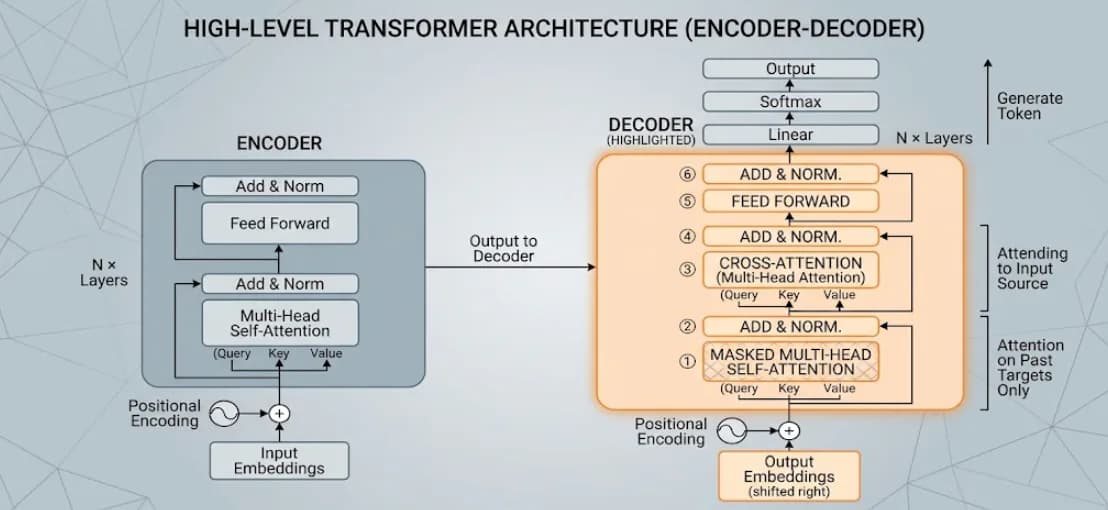
A transformer is often explained as a stack of attention layers, treated as if serving the model is an entirely separate infrastructure problem. In reality, the two are inseparable. A model's mathematical architecture directly determines what data must be saved during text generation—and that data dictates memory capacity, server batching behavior, latency, and ultimately your cloud bill.
This is the first article in a three-part series that follows a decoder-only transformer from language modelling to production serving. Before we can solve the memory bottlenecks (Part 2) or scale the engine to handle thousands of concurrent users (Part 3), we must understand the engine itself. In this post, we will strip away the magic and look at the exact mechanics of how a prompt becomes a predicted token, following the data through tokenization, causal self-attention, and feed-forward layers.
The content is structured as:
- The mechanics of next-token prediction
- Why transformers?
- Decoder architecture
- Where inference begins
A separate notebook series implements the same ideas in PyTorch and then carries the model into serving experiments.
1. The mechanics of next-token prediction
Consider a short sequence:
The company reported higher revenue.
A language model learns from this sequence by repeatedly answering one question:
Given the tokens seen so far, which token should come next?
The same sentence creates several training examples:
| Context available to the model | Target token |
|---|---|
The | company |
The company | reported |
The company reported | higher |
The company reported higher | revenue |
The company reported higher revenue | . |
This next-token task is the foundation for both training and generation. For every position, the model learns a probability distribution for the next token:
For example, after the context The company reported higher, the model might
assign different probabilities to revenue, earnings, costs, and many other
tokens. Training encourages it to assign more probability to the token that
actually appears next.
Repeating this task across large amounts of text helps the model learn patterns in language, documents, and code. These patterns are distributed across many internal weights rather than stored as individual sentences in one location.
Next-token prediction has a strict information rule: the prediction at position may use the current context and earlier tokens, but not later tokens. Regardless of the underlying architecture, the model must be prevented from looking ahead at future information during training. The training sequence supplies both inputs and targets simply by shifting the same tokens by one position:
Input:   The company reported higher revenue
Target:      company reported higher revenue .
For tokens , the cross-entropy objective is:
The model compares its predictions with the actual next tokens, adjusting its weights when it guesses incorrectly. The fundamental engineering challenge here is speed: because each position only relies on earlier tokens, the predictions for an entire training sequence could theoretically be calculated simultaneously. How a model actually achieves that parallelism without violating the strict "no looking ahead" rule is what separates modern architectures from the previous generation of neural networks.
2. Why transformers?
Before 2017, sequence modelling was dominated by recurrent neural networks (RNNs) and LSTMs. They pass information through recurrent state updates, meaning they must process text strictly word-by-word. This creates a hard dependency between consecutive positions, which severely limits parallelism during training and forces distant tokens to communicate through a long, easily degraded information path.
The transformer replaced recurrent state updates with self-attention as its primary mechanism for exchanging information across positions. Attention gives each token a direct, instant mathematical path to the earlier context it is allowed to use, completely removing the step-by-step bottleneck. As a result, all known positions in a massive training sequence can be processed in parallel.
The original architecture introduced in Attention Is All You Need paired an encoder stack with a decoder. However, many general-purpose generative LLMs today have dropped the encoder entirely. To maintain the strict "no looking ahead" rule while still processing tokens in parallel, a decoder-only transformer relies on a causal mask— a mathematical filter that actively hides future tokens from earlier positions during self-attention.
Depending on how this visibility is restricted, the transformer architecture dictates its ideal use case:
| Architecture | Self-attention visibility | Typical use |
|---|---|---|
| Encoder-only | Each token can attend to every input token, both earlier and later | Classification, retrieval, token labelling, span extraction |
| Encoder–decoder | Encoder tokens attend in both directions; decoder tokens attend only to themselves and earlier output tokens, while also attending to the encoded input | Translation, summarisation, structured transformation |
| Decoder-only | Each token attends only to itself and earlier tokens; later positions are hidden by a causal mask | Completion, conversation, instruction following, open-ended generation |
3. Decoder Architecture
To understand how a model actually generates text, we first need to look at the end-to-end anatomy of the process. Think of this as the roadmap of a single prompt traveling through the model's architecture.
The complete generation path is:
Prompt text
    ↓
Tokenizer and token IDs
    ↓
Input representations and positional information   (Section 3.1)
    ↓
Stack of decoder transformer blocks                (Section 3.2)
    ├── RMSNorm and residual connections         (Section 3.2.3)
    ├── Causal self-attention                    (Section 3.2.1)
    └── Gated feed-forward network               (Section 3.2.2)
    ↓
Final normalisation and vocabulary projection      (Section 3.3)
    ↓
Next-token probabilities                           (Section 3.3)
    ↓
Selected token, appended to the prompt             (Section 3.3)
The following subsections will progressively unpack this pipeline, starting from the initial representations that enter the model and moving all the way through to the final token prediction.
3.1 Input representations and positional information
Text does not enter the model as words. A tokenizer divides it into tokens from a fixed vocabulary and maps each token to an integer ID. Depending on the tokenizer, a token may represent a word, a subword, punctuation, whitespace, or a byte-level fragment.
Each ID acts as an index to retrieve a specific row from a learned vocabulary matrix (often called an embedding table). If the vocabulary has 50,000 tokens, this matrix has the shape [50000, d_model]. This lookup operation maps the integer ID to a continuous embedding vector of width . For batch size and sequence length , the initial residual stream has shape:
For example,
Batch size:       2
Sequence length:  128 tokens
Model width:      4,096 values per token

Residual-stream shape: [2, 128, 4,096]
Self-attention by itself has no notion of token order. The original transformer added fixed sinusoidal positional encodings to token embeddings. Many current decoders instead use Rotary Position Embeddings (or RoPE). RoPE rotates pairs of query and key coordinates according to token position, making relative position affect their dot product without adding a separate vector to the residual stream.
Comparison of Sinusoidal encoding and RoPE
| Property | Sinusoidal encoding | RoPE |
|---|---|---|
| Applied to | Token embeddings/residual input | Queries and keys |
| Operation | Addition | Rotation |
| Position representation | Primarily absolute, with recoverable relative relationships | Relative displacement appears directly in query-key scores |
| Learned parameters | None in the standard form | None in the standard form |
| Applied to values | Indirectly, because position is added before projections | No |
| Common usage | Original transformer and some later models | Many modern decoder-only LLMs |
RoPE is normally a deterministic transformation rather than a learned projection matrix. Its configuration still matters: base frequencies (where different vector dimensions rotate at progressively slower speeds to encode both fine-grained and coarse-grained distances), scaling method, and maximum context assumptions affect long-context behaviour.
RoPE
RoPE does not add a position vector to the token embedding. Instead, it rotates pairs of coordinates in the query and key vectors. The processing order is:
Token representation
        ↓
Q and K projections
        ↓
Position-dependent rotation
        ↓
Attention scores
For one two-dimensional pair, RoPE applies a rotation matrix:
At position , a query vector is rotated by an angle based on :
At position , a key is rotated by its corresponding angle:
Because rotation matrices are orthogonal, the dot product of the rotated query and key simplifies to isolate the relative distance:
This is RoPE’s most important property: the query-key score naturally and mathematically contains information about the relative displacement .
In other words, attention can distinguish:
The matching token is 1 position earlier.
The matching token is 100 positions earlier.
even when the token content is the same.
Why rotate only Q and K?
- Query (Q): What am I looking for?
- Key (K): What information does this token offer?
- Value (V): The actual information to retrieve.
RoPE rotates Q and K so their matching score includes how far apart the tokens are. V is not rotated because it carries the content after the match is decided.
RoPE also preserves vector magnitude because rotation changes direction but not length.
3.2 Inside the transformer block
The token representations pass through a sequence of transformer blocks:
Initial representations X₀
        ↓
Transformer block 0
        ↓
Transformer block 1
        ↓
       ...
        ↓
Transformer block L−1
        ↓
Final representations Xᴸ
Every block shares the same structural blueprint but contains its own unique learned weights. Each block reads the current residual stream, injects new contextual information, and passes the updated representations up to the next block. Through this sequence, the model's understanding of the text is progressively refined across the stack.
A modern pre-norm decoder block relies on three fundamental mechanisms:
- Causal self-attention: which routes and mixes information across different token positions.
- Feed-forward network (MLP): which transforms the representation at each position independently.
- RMSNorm and residual connections: which stabilize the learning process and ensure information flows cleanly through the deep network without degrading.
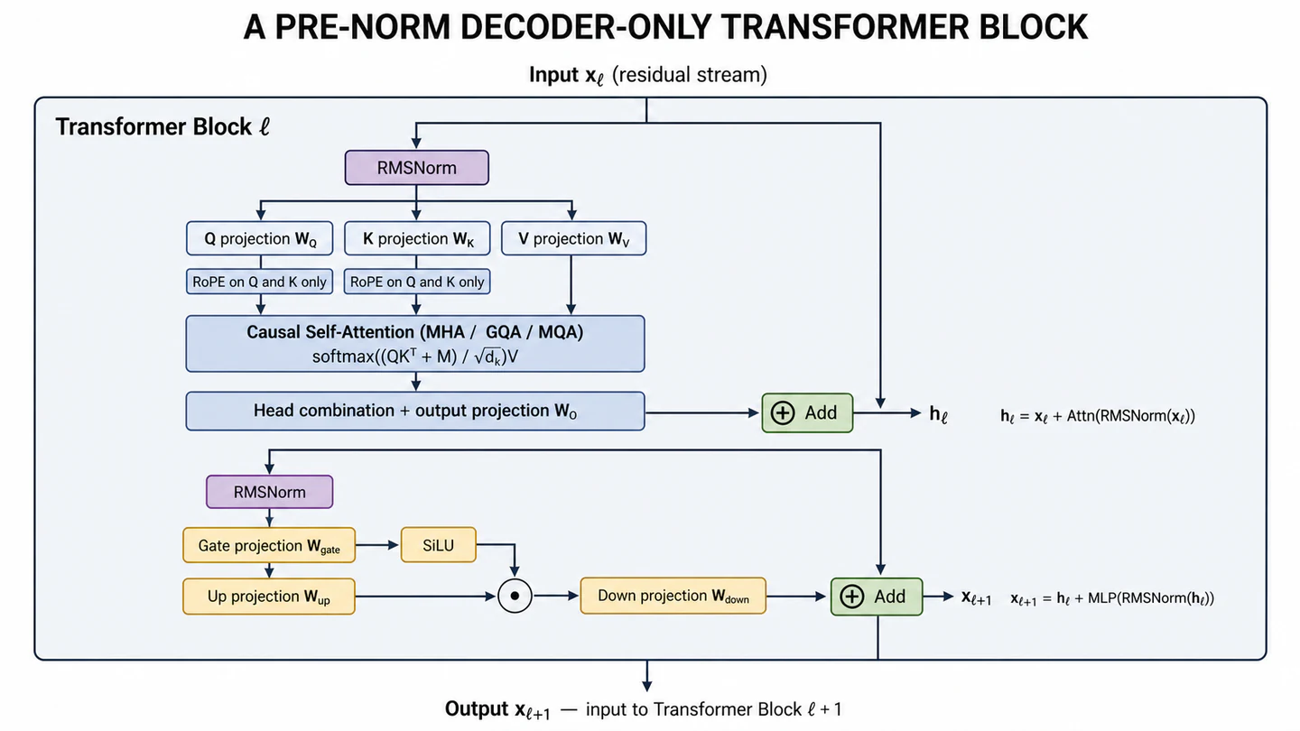
The block receives a residual stream and produces the input to the next block, . By stacking many blocks with different learned parameters, the model builds deep, complex representations.
The mathematical flow through layer ties these three mechanisms together:
xₗ
 ↓ RMSNorm → Attention update → Residual addition
hₗ
 ↓ RMSNorm → MLP update → Residual addition
xₗ₊₁
Here, is the block input, is the intermediate representation after the attention update, and is the final block output passed to the next layer in the stack.
3.2.1 Causal self-attention
Self-attention is the mechanism that decides which tokens in the context should influence the current token. To achieve this, it relies on three elements: Queries, Keys, and Values.
Queries, Keys, and Values
For a sequence of hidden states , the attention layer creates queries, keys, and values through learned linear projections:
These three representations serve distinct roles:
- A query describes what the current token is looking for;
- A key describes what a token offers for matching; and
- A value carries the information returned when that token receives attention weight.
The core operation is scaled dot-product attention:
The query-key dot product () measures the compatibility between tokens. Dividing this score by prevents the magnitude of the dot product from growing too large with the head width. Without this scaling, the values would push the softmax function into an extremely saturated regime, leading to vanishing gradients during training.
The Causal Mask
In the formula above, represents the causal mask. To enforce the strict autoregressive rule (no looking into the future), entries in representing future positions are set to before softmax is applied.
Because the softmax of is zero, token can attend to itself and earlier positions (), but its attention weight for any future position () is zeroed out. This mask is what allows the transformer to process all positions in a training sequence simultaneously while preserving the integrity of next-token prediction.
Note: Attention is best understood as contextual information routing, not a strict database lookup. A high attention score does not act as definitive proof for why the model produced a specific answer. A useful representation emerges across many heads and layers, and it should not be assumed that one attention head corresponds cleanly to one human-interpretable function.
Multi-head and grouped-query attention
Instead of applying one massive attention operation across the full model width, multi-head attention splits the queries, keys, and values into smaller, parallel "heads." This allows the model to attend to different types of relationships simultaneously—for example, one head might track grammatical structure while another resolves pronoun references.
Each head performs attention in its own learned subspace. The results are then concatenated and passed through a final projection matrix :
Concatenation places the head outputs side by side. The learned matrix then mixes the information across those distinct head dimensions and maps the combined result back to the original model width (). This step is crucial: the attention output must match the width of the residual stream before the two can be added together. Even if the concatenated width already equals , ensures the model learns how to optimally combine the different heads rather than leaving them as separate groups of features.
Not every modern decoder uses a strict 1:1 ratio of query heads to key-value heads. Grouped-query attention (GQA) is an architectural variant that allows several query heads to share a single key-value head.
Grouped-query attention (GQA)
Grouped-query attention lets several query heads share the same key and value heads. For example:
8 query heads
2 key/value heads

Query heads 1–4 → share KV head 1
Query heads 5–8 → share KV head 2
Comparison of architectures:
- Multi-head attention (MHA): Every query head has its own unique K and V.
- Grouped-query attention (GQA): A group of query heads shares K and V.
- Multi-query attention (MQA): All query heads share a single K and V.
Why do this?
The main benefit of GQA is a significantly smaller KV cache and reduced memory bandwidth bottlenecks during generation. GQA preserves more modelling capacity and output quality than sharing a single KV head (MQA), making it the standard practical compromise between text quality and serving efficiency in modern open-weights models.
This is a critical optimization choice that has major consequences for production serving, which will be explored in depth later in this series.
3.2.2 Gated feed-forward network (MLP)
While self-attention routes information between different positions (inter-token), the feed-forward network (or MLP), transforms the representation at each position completely independently (intra-token) using the same shared learned weights.
The original transformer used two linear projections separated by a standard ReLU activation. However, most modern decoders have adopted a "gated" architecture, such as SwiGLU:
In this design, each token enters as a vector of values. The MLP temporarily expands it into a much wider feature space, , processes it, and compresses it back down:
Input (x):                 d_model values
                                ↓
Up projection (W_up):      d_ff candidate features
Gate projection (W_gate):  d_ff gate values
                                ↓
Activation (SiLU):         Applies non-linearity to the gate
                                ↓
Multiplication (⊙):        Element-wise multiplication
                                ↓
Down projection (W_down):  d_model values
Notice that the network creates two expanded vectors of the exact same size ():
- The up projection () creates the raw candidate features.
- The gate projection () decides how strongly each candidate feature should pass through to the next stage.
The SiLU (Sigmoid Linear Unit) activation transforms the gate projection into a set of learned "dimmer switches." These two wide vectors are then multiplied together one value at a time ():
The dimmer switches strengthen useful features and suppress less useful ones. Finally, the down projection () compresses these selected features back to the original width, allowing the result to be cleanly added back into the residual stream. (Note: this "expansion" strictly refers to the number of features per token, not the number of tokens in the sequence).
Because of this massive internal expansion space, MLPs frequently contain the largest share of a dense transformer's total parameters—though the exact percentage depends on the model's width, vocabulary size, and whether it uses sparse experts (MoE). Research often associates these dense MLP layers with the model's factual recall and associative memory, though it is important to remember that model knowledge is holistic and does not live exclusively in one isolated component.
3.2.3 RMSNorm and residual connections
Modern decoder families commonly use a "pre-normalization" architecture: the input is normalized immediately before passing through a transformation, while an unnormalized residual path bypasses it entirely.
Using RMSNorm, the mathematical flow for one complete block can be written as:
RMSNorm rescales the input to keep activation magnitudes stable before the attention or MLP layers process them. The residual connection (the and ) acts as an information highway. It preserves the existing representation, allowing the attention and MLP layers to add their new results as updates, rather than completely replacing the original information. (This is exactly why both attention and the MLP must project their final outputs back to the model width —the dimensions must match so they can be added directly back into the residual stream).
While older models like the original transformer used LayerNorm, modern decoders largely prefer RMSNorm. LayerNorm centers (subtracts the mean) and rescales activations; RMSNorm only rescales them. Dropping the mean-centering step provides a noticeable boost to computational speed and efficiency during training and inference without degrading the model's performance.
3.3 Vocabulary projection and token selection
After the sequence passes through the final transformer block (), the residual stream holds a deeply contextualized representation for every token in the prompt. However, because next-token prediction operates strictly left-to-right, the model only looks at the representation of the very last token in the sequence to determine what comes next.
Final normalization and projection
This final vector first passes through one last RMSNorm layer to stabilize its values. Then, it hits the language modeling head (or un-embedding matrix). This learned projection matrix maps the vector from the internal model width back out to the full vocabulary size.
Final token representation:  [d_model]
                                ↓
Vocabulary projection:       [vocab_size]
If the model has a vocabulary of 50,000 tokens, this projection outputs a vector of 50,000 raw, unnormalized scores known as logits.
Next-token probabilities
Because logits can be any real number (positive or negative), they must be converted into a valid probability distribution. The model applies a softmax function:
This forces all 50,000 scores into a range between 0 and 1, ensuring they sum perfectly to 1.0 (or 100%). At this moment, the model has completed its forward pass. It has assigned a probability to every possible word, subword, and punctuation mark it knows.
Selection and the autoregressive loop
The model itself does not strictly choose the next token; it only provides the probabilities. The actual selection is dictated by the decoding strategy:
- Greedy decoding: Simply selects the token with the highest probability (the ).
- Sampling (Temperature, Top-P, Top-K): Adjusts the logits to make the distribution flatter (more creative) or sharper (more focused), and then randomly selects a token based on those weighted probabilities.
Once a token is chosen, the loop closes: the new token is appended to the original prompt, forming a new, slightly longer sequence. This new sequence is fed directly back into the tokenizer at Step 1, and the entire massive architectural process repeats to predict the token after that.
4. Where inference begins
The architecture we just explored explains exactly what must happen to execute a single forward pass. But production serving introduces an entirely different challenge:
How can a system generate many tokens, for many concurrent requests, without repeatedly recomputing the mathematical history of every prompt?
The next article, LLM Inference: How KV Caching and PagedAttention Save LLM Inference, separates the generation process into prefill and decode phases, exposing exactly how the self-attention state transforms from a theoretical mechanism into a massive production memory bottleneck.
Transformer 常被簡化為「多層注意力機制」,模型部署則經常被視為另一個獨立的基礎設施議題。實際上,兩者密切相關:模型的數學架構會直接決定生成文字時必須保留哪些狀態,而這些狀態又會影響記憶體需求、批次排程、延遲與整體運算成本。
本文是三部曲的第一篇,將從語言建模出發,解析純解碼器 Transformer 的核心架構。在進一步討論記憶體瓶頸(第二篇)與大規模模型服務(第三篇)之前,我們先追蹤資料如何流經 tokenization(分詞)、因果自注意力與前饋網路,釐清提示詞如何轉換為下一個 token 的機率分布。
本文結構如下:
另有一系列獨立的 notebook,會用 PyTorch 實作同樣的概念,並進一步將模型帶入服務端的實驗。
1. 下一個 token 預測的運作機制
來看一個簡短的序列:
The company reported higher revenue.
語言模型會透過反覆回答同一個問題,從這個序列中學習:
根據目前為止看到的 token,下一個 token 應該是什麼?
同一個句子,會產生好幾筆訓練樣本:
| 模型可取用的上下文 | 目標 token |
|---|---|
The | company |
The company | reported |
The company reported | higher |
The company reported higher | revenue |
The company reported higher revenue | . |
這個「預測下一個 token」的任務,正是訓練與生成兩者共同的基礎。對序列中的每一個位置,模型都會學習一個關於下一個 token 的機率分布:
舉例來說,在看過 The company reported higher 這段上下文之後,模型可能會為 revenue、earnings、costs 等許多不同的 token 分配不同的機率。訓練的作用,就是鼓勵模型把更高的機率,分配給實際上真正接下來出現的那個 token。
在大量文本上反覆執行這項任務,模型便能學習語言、文件與程式碼中的統計規律。這些能力分散在模型的眾多權重之中,並不是將個別句子原封不動地存放在某個單一位置。
下一個 token 預測,遵循一條嚴格的資訊規則:位置 的預測,只能使用目前的上下文與更早之前的 token,絕不能用到後面的 token。無論底層架構為何,模型在訓練時都必須被禁止「偷看」未來的資訊。訓練序列只需將同一串 token 整體位移一個位置,就能同時提供輸入與目標:
Input:   The company reported higher revenue
Target:      company reported higher revenue .
對於 token 序列 ,其交叉熵目標函數為:
訓練時,模型會比較預測分布與實際的下一個 token,再根據誤差更新權重。核心的工程問題在於:如何在禁止每個位置使用未來資訊的前提下,同時計算序列中所有位置的預測。能否有效完成這項平行運算,正是 Transformer 與上一代序列模型的重要差異。
2. 為什麼是 Transformer?
在 2017 年之前,循環神經網路(RNN)與 LSTM 是序列建模的主流。它們透過反覆更新隱藏狀態來傳遞資訊,因此必須依序處理文本。這種前後相依的計算方式限制了訓練的平行化程度,也讓相距較遠的 token 必須經過較長的資訊路徑才能互相影響。
Transformer 以自注意力機制取代循環式的狀態更新,作為不同位置交換資訊的主要方式。在純解碼器模型中,每個 token 都能直接連結到因果遮罩允許參照的較早位置。由於訓練資料中的所有 token 都已知,模型可以平行計算序列中各個位置的表示,而不必像 RNN 一樣逐步等待前一個位置完成。
〈Attention Is All You Need〉這篇論文提出的原始架構,是將一組編碼器與一個解碼器搭配使用。然而,今日許多通用型的生成式 LLM,都已經完全捨棄了編碼器。純解碼器 Transformer 為了在平行處理 token 的同時,仍然維持「禁止偷看未來」這條嚴格規則,仰賴的是因果遮罩——一種在自注意力運算中,主動將未來的 token 隱藏起來、不讓較早位置看見的數學濾網。
依照這種可見範圍受限制的方式不同,Transformer 架構也各自適合不同的使用情境:
| 架構 | 自注意力可見範圍 | 典型用途 |
|---|---|---|
| 純編碼器 | 每個 token 都能關注到輸入中所有的 token,無論在它之前或之後 | 分類、檢索、token 標註、片段擷取 |
| 編碼器-解碼器 | 編碼器的 token 可雙向關注;解碼器的 token 則只能關注自己與更早的輸出 token,同時也會關注已編碼的輸入內容 | 翻譯、摘要、結構化轉換 |
| 純解碼器 | 每個 token 只能關注自己與更早的 token;較晚的位置會被因果遮罩隱藏 | 文字接龍、對話、指令遵循、開放式生成 |
3. 解碼器架構
要理解模型如何生成文字,可以先從端到端的資料流程著手,觀察提示詞進入模型後,依序經過哪些轉換。
完整的生成路徑如下:
提示詞文字
    ↓
Tokenizer 與 token ID
    ↓
輸入表示與位置資訊                    (第 3.1 節)
    ↓
多層解碼器 Transformer block          (第 3.2 節)
    ├── RMSNorm 與殘差連接           (第 3.2.3 節)
    ├── 因果自注意力機制             (第 3.2.1 節)
    └── 閘控前饋網路                 (第 3.2.2 節)
    ↓
最終正規化與詞彙表投影                (第 3.3 節)
    ↓
下一個 token 的機率                   (第 3.3 節)
    ↓
選出 token,附加至既有序列             (第 3.3 節)
接下來的小節,會循序漸進地拆解這整條流程,從進入模型的最初表示開始,一路講到最終的 token 預測。
3.1 輸入表示與位置資訊
文字不是以完整「詞語」為固定單位進入模型。Tokenizer(分詞器)會根據既定詞彙表將文字切分為 token,並把每個 token 映射為整數 ID。視 tokenizer 的設計而定,一個 token 可能代表完整詞語、子詞、標點、空白或位元組層級的片段。
每個 ID 都是索引,用來從模型學習得到的嵌入表中取出對應的一列。如果詞彙表包含 50,000 個 token,矩陣形狀就是 [50000, d_model]。這項查找會將整數 ID 轉換為寬度為 的連續向量。對於批次大小 與序列長度 ,初始殘差流的形狀為:
舉例來說,
批次大小:           2
序列長度:           128 個 token
模型寬度:           每個 token 4,096 個數值

殘差流形狀:[2, 128, 4,096]
自注意力運算本身無法辨識 token 的排列順序。原始 Transformer 會在 token 嵌入上加入固定的正弦位置編碼;許多現代解碼器則採用旋轉位置嵌入(Rotary Position Embeddings,RoPE)。RoPE 會根據 token 的位置,旋轉 Query 與 Key 中成對的維度,使相對位置直接影響兩者的點積結果,而不必在殘差流中額外加入位置向量。
正弦位置編碼與 RoPE 的比較
| 特性 | 正弦位置編碼 | RoPE |
|---|---|---|
| 作用對象 | Token 嵌入/殘差流輸入 | Query 與 Key |
| 運算方式 | 相加 | 旋轉 |
| 位置表示方式 | 主要為絕對位置,但相對關係仍可還原 | 相對位移直接反映在 query-key 分數中 |
| 是否有學習參數 | 標準形式下沒有 | 標準形式下沒有 |
| 是否作用於 Value | 間接影響,因為位置資訊在投影之前就已加入 | 否 |
| 常見使用場合 | 原始 Transformer 及部分後續模型 | 許多現代的純解碼器 LLM |
RoPE 通常是一種確定性的變換,而不是一個學習得來的投影矩陣。不過,它的設定仍然重要:基礎頻率(不同的向量維度,會以逐漸放慢的速度旋轉,藉此同時編碼精細與粗略的距離資訊)、縮放方法,以及對最大上下文長度的假設,都會影響模型在長上下文情境下的表現。
RoPE 的技術細節
RoPE 並不會把位置向量加到 token 嵌入上,而是旋轉 query 與 key 向量中成對的座標。其處理順序為:
Token 表示
        ↓
Q 與 K 投影
        ↓
依位置而定的旋轉
        ↓
注意力分數
對於單一一組二維的座標對,RoPE 會套用一個旋轉矩陣:
在位置 上,query 向量會依據 旋轉一個對應的角度:
在位置 上,key 則會旋轉其對應的角度:
由於旋轉矩陣具有正交性,旋轉後的 query 與 key 做點積時,會化簡成只留下相對距離的形式:
這正是 RoPE 最重要的特性:query-key 分數,會在數學上自然而然地包含相對位移 的資訊。
換句話說,注意力機制能夠分辨:
匹配的 token 在 1 個位置之前。
匹配的 token 在 100 個位置之前。
即使 token 的內容完全相同,也能做出這樣的區分。
為什麼只旋轉 Q 和 K?
- Query(Q):我正在尋找什麼?
- Key(K):這個 token 能提供什麼資訊?
- Value(V):真正要被取用的實際資訊。
RoPE 只旋轉 Q 與 K,讓兩者的匹配分數能反映出 token 之間相隔多遠。V 則不旋轉,因為它承載的是匹配結果確定「之後」才會用到的實際內容。
此外,RoPE 會保留向量的長度(也就是向量的大小或範數),因為旋轉只改變方向,不改變向量本身的尺度。
3.2 深入 Transformer Block 內部
Token 的表示,會依序通過一連串的 Transformer block:
初始表示 X₀
        ↓
Transformer block 0
        ↓
Transformer block 1
        ↓
       ...
        ↓
Transformer block L−1
        ↓
最終表示 Xᴸ
每個 block 都採用相同的結構,但擁有各自獨立的可學習權重。它會讀取目前的殘差流、加入新的上下文資訊,再把更新後的表示傳遞給下一個 block。經過多層轉換後,模型的上下文表示會逐步精煉。
一個現代的 pre-norm 解碼器 block,仰賴三個基本機制:
- 因果自注意力機制:負責在不同 token 位置之間傳遞並混合資訊。
- 前饋網路(MLP):針對每個位置獨立進行轉換。
- RMSNorm 與殘差連接:穩定數值與梯度,使資訊能順利通過深層網路。
這個 block 接收殘差流 作為輸入,並產生下一個 block 的輸入 。透過堆疊許多個各自擁有不同學習參數的 block,模型得以建構出既深且複雜的表示。
第 層的數學流程,將這三個機制串連在一起:
xₗ
 ↓ RMSNorm → 注意力更新 → 殘差相加
hₗ
 ↓ RMSNorm → MLP 更新 → 殘差相加
xₗ₊₁
這裡, 是 block 的輸入, 是經過注意力更新後的中間表示,而 則是傳遞給堆疊中下一層的最終 block 輸出。
3.2.1 因果自注意力機制
自注意力機制會計算上下文中各個 token 對目前位置的影響程度。這項運算包含三種表示:Query、Key 與 Value。
Query、Key 與 Value
對於一串隱藏狀態 ,注意力層會透過學習得來的線性投影,產生 query、key 與 value:
這三種表示,各自扮演不同的角色:
- Query 描述目前這個 token 要尋找哪些特徵;
- Key 描述某個 token 可供比對的特徵;
- Value 承載注意力權重確定後,實際要彙整的資訊。
核心運算是縮放點積注意力(scaled dot-product attention):
Query 與 key 的點積()衡量的是 token 之間的相容程度。將這個分數除以 ,能避免點積的量級隨著 head 寬度增加而變得過大。若沒有這個縮放步驟,這些數值會把 softmax 函數推向極度飽和的區域,導致訓練時出現梯度消失的問題。
因果遮罩
在上面的公式中, 代表因果遮罩。為了強制執行嚴格的自迴歸規則(禁止窺看未來), 中代表未來位置的項目,在套用 softmax 之前,會先被設為 。
由於 經過 softmax 後會變成零,token 可以關注自己與更早的位置(),但對任何未來位置()的注意力權重都會被歸零。正是這個遮罩,讓 Transformer 得以同時處理訓練序列中的所有位置,同時仍完整保留下一個 token 預測的正確性。
注意力機制比較適合被理解為「上下文資訊的路由」,而不是事實資料庫或可直接解讀的推理軌跡。高注意力分數只能表示某次運算中的關聯強度,不能單獨證明模型為何產生特定答案。模型的表示通常分散在多個 head 與多個層次之中,不應假設單一注意力 head 必然對應某項人類可理解的功能。
多頭注意力與分組查詢注意力
多頭注意力(multi-head attention)不會只在完整模型寬度上執行一次注意力運算,而是將 Query、Key 與 Value 拆分為多個較小、可平行運算的 head。不同 head 可以學習不同類型的關係;例如,有些 head 可能較常捕捉語法結構,有些則可能與代名詞指涉有關,但這些功能通常不是完全獨立或固定的。
每個 head 都在自己學習得來的子空間中執行注意力運算。這些結果接著會被串接起來,再通過最終的投影矩陣 :
串接會把各個 head 的輸出並排組合,再由可學習的輸出投影矩陣 混合不同 head 的資訊,並將結果映射回模型寬度 。這一步很重要:首先,注意力輸出的維度必須與殘差流一致,兩者才能相加;其次,即使串接後的寬度已等於 , 仍可學習如何重新組合各個 head 的特徵,而不是讓它們彼此獨立地保留在不同區段。
並非每個現代解碼器,都採用嚴格 1:1 比例的 query head 對 key-value head。分組查詢注意力(GQA)是一種架構上的變體,允許好幾個 query head 共用同一個 key-value head。
分組查詢注意力(GQA)的技術細節
分組查詢注意力,讓好幾個 query head 共用相同的 key 與 value head。舉例來說:
8 個 query head
2 個 key/value head

Query head 1–4 → 共用 KV head 1
Query head 5–8 → 共用 KV head 2
架構比較:
- 多頭注意力(MHA):每個 query head 都各自擁有獨一無二的 K 與 V。
- 分組查詢注意力(GQA):一組 query head 共用 K 與 V。
- 多查詢注意力(MQA):所有 query head 共用單一一組 K 與 V。
為什麼要這麼做?
GQA 最主要的好處,是能大幅縮小 KV 快取,並降低生成階段的記憶體頻寬瓶頸。相較於只共用單一 KV head 的 MQA,GQA 保留了更多的建模能力與輸出品質,因此成為現代開放權重模型中,在文字品質與服務效率之間,最常見的實務折衷方案。
這項架構選擇會直接影響推論時的 KV 快取大小與記憶體頻寬需求,本系列後續文章將進一步說明。
3.2.2 閘控前饋網路(MLP)
自注意力機制負責在不同位置之間(token 與 token 之間)傳遞資訊,而前饋網路(或稱 MLP),則是使用同一組共享的學習權重,完全獨立地(在單一 token 內部)轉換每個位置的表示。
最初的 Transformer,使用的是兩個線性投影中間夾著一個標準 ReLU 激活函數。然而,如今大多數現代解碼器,都已改採「閘控」架構,例如 SwiGLU:
在這種設計中,每個 token 都是以一個 維的向量進入。MLP 會先暫時將它擴展到寬得多的特徵空間 ,進行處理後,再壓縮回原本的維度:
輸入(x):                  d_model 個數值
                                ↓
Up projection(W_up):      d_ff 個候選特徵
Gate projection(W_gate):  d_ff 個閘門數值
                                ↓
激活函數(SiLU):            對閘門施加非線性
                                ↓
逐元素相乘(⊙):             逐一元素相乘
                                ↓
Down projection(W_down):  d_model 個數值
這個網路會產生兩個維度相同(皆為 )的擴展向量:
- Up projection()產生候選特徵。
- Gate projection()決定每個候選特徵要以多大程度傳遞到下一階段。
SiLU(Sigmoid Linear Unit)激活函數會將 gate projection 轉換為可學習的閘門係數,接著與候選特徵逐元素相乘():
這些閘門係數會放大、保留或抑制不同特徵。最後,down projection()把篩選後的特徵投影回原本的 寬度,使結果能夠加回殘差流。這裡的「擴展」是指增加每個 token 的特徵維度,而不是增加序列中的 token 數量。
正因為內部有這麼龐大的擴展空間,MLP 往往佔了一個密集型(dense)Transformer 總參數量中最大的一部分——不過確切比例,仍取決於模型的寬度、詞彙表大小,以及是否採用了稀疏專家(MoE)架構。研究常將這些密集的 MLP 層,與模型的事實記憶及聯想記憶連結在一起,但仍要記得,模型的知識是整體性的,並不會只獨立存在於某一個孤立的元件之中。
3.2.3 RMSNorm 與殘差連接
現代的解碼器家族,普遍採用「pre-normalization」(前置正規化)架構:輸入在進入某個轉換之前,會先立即被正規化,同時有一條未經正規化的殘差路徑,完全繞過這個轉換。
使用 RMSNorm 時,一個完整 block 的數學流程可以寫成:
RMSNorm 會重新縮放輸入,使激活值的量級在進入注意力層或 MLP 前保持穩定。殘差連接(也就是 與 )則保留原有表示,讓注意力層與 MLP 將新結果當作增量更新疊加,而不是完全取代既有資訊。這也是注意力與 MLP 最終都必須將輸出投影回模型寬度 的原因:維度一致後,結果才能直接加回殘差流。
原始 Transformer 使用 LayerNorm,許多現代解碼器則採用 RMSNorm。LayerNorm 會將激活值置中(減去平均值)並重新縮放;RMSNorm 只根據均方根重新縮放,不執行置中。它的計算較簡化,實際效益則取決於模型架構與核心實作。
3.3 詞彙表投影與 token 選擇
序列通過最後一個 transformer block()之後,殘差流中保存著提示詞裡每一個 token、經過深度上下文化後的表示。不過,由於下一個 token 預測嚴格依由左至右的順序進行,模型在決定接下來會出現什麼時,只會參考序列中最後一個 token 的表示。
最終正規化與投影
這個最終向量,會先通過最後一層 RMSNorm,穩定其數值,接著送進語言模型頭(language modeling head,又稱反嵌入矩陣)。這個學習得來的投影矩陣,會把向量從模型內部的寬度,映射回完整的詞彙表大小。
最終 token 表示:              [d_model]
                                ↓
詞彙表投影:                   [vocab_size]
如果模型的詞彙表有 50,000 個 token,這個投影就會輸出一個由 50,000 個原始、未正規化分數組成的向量,這些分數稱為 logits。
下一個 token 的機率
由於 logits 可以是任何實數(正數或負數),必須先轉換成合法的機率分布。模型會套用 softmax 函數:
這會強制把全部 50,000 個分數,壓縮到 0 到 1 之間的範圍,並確保它們的總和恰好等於 1.0(也就是 100%)。到了這一刻,模型已經完成了一次前向傳播,為它所知道的每一個可能的詞、子詞與標點符號,都分配好了一個機率。
選擇與自迴歸迴圈
嚴格來說,模型本身並不會挑選下一個 token,它只負責提供機率。真正的選擇,是由解碼策略來決定的:
- 貪婪解碼(Greedy decoding):直接選擇機率最高的那個 token(也就是 )。
- 採樣(溫度、Top-P、Top-K):調整 logits,讓機率分布變得更平(更有創意)或更尖銳(更聚焦),接著再依照這些加權後的機率,隨機選出一個 token。 一旦選定 token,對應的 token ID 就會附加到既有序列,模型再以更新後的序列執行下一輪前向傳播,預測後續 token。實際的推論系統通常會利用 KV 快取保留先前計算結果,避免每一輪都重新處理完整序列;這正是下一篇文章的主題。
4. 推論從這裡開始
我們剛才探討的架構,精確地說明了執行單一次前向傳播究竟需要發生哪些事。但正式上線服務,帶來的是一個截然不同的挑戰:
一個系統要如何同時為大量請求生成 token,又不必反覆計算每段提示詞已處理過的內容?
下一篇文章〈LLM 推論:KV 快取、FlashAttention 與 PagedAttention〉會把生成過程拆分成預填充(prefill)與解碼(decode)兩個階段,說明自注意力所產生的狀態,如何成為正式服務中的主要記憶體負擔。