LLM Inference: How KV Caching and PagedAttention Save LLM InferenceLLM 推論:KV 快取、FlashAttention 與 PagedAttention
When models scale, memory becomes the enemy. A deep dive into the engineering behind prefill and decode bottlenecks, and the memory management breakthroughs that make real-time generative serving feasible.解析預填充與解碼的不同瓶頸,以及 KV 快取、FlashAttention、PagedAttention 與模型壓縮如何改善 LLM 推論效率。
This is the second article in a three-part series. Our first installment, LLM Pretrain: Anatomy of a Decoder-Only Transformer, explored the mathematical mechanics of how a model turns raw text into next-token probabilities.
Pretraining is only the beginning. Once training finishes and the model weights are frozen, the challenge shifts from learning to execution. In production, the model processes dynamic prompts where every newly generated token must be fed back into the model to extend its growing attention history. Each request generates tokens sequentially and retains its own growing state, transforming the core problem from pure training compute into one of memory bandwidth, hardware efficiency, and real-time state manipulation.
| Concern | Pretraining | Inference |
|---|---|---|
| Input | Large batches of complete sequences | Dynamic prompts arriving over time |
| Goal | Minimise next-token loss | Generate useful tokens within memory and latency constraints |
| State | Weights, gradients, optimiser state, activations | Weights and per-request KV cache |
| Parallelism | Many sequence positions processed together | Prefill is parallel; decode advances autoregressively |
| Memory pressure | Parameters, gradients, optimiser, activations | Parameters, KV cache, hardware workspaces |
| Primary metrics | Training tokens/s, convergence, utilisation | Time to First Token (TTFT), inter-token latency, throughput |
(Note: Broader production serving architecture, request scheduling, and Service Level Objectives will be explored in detail in the final article of this series).
In this article, we look at why that shift makes LLM inference fundamentally harder than training, and how specific systems-level breakthroughs—like KV caching, FlashAttention, PagedAttention, and model compression—tame the growing attention state and bandwidth bottlenecks to keep execution fast and efficient.
The content is structured as:
- The two phases of inference: prefill and decode
- KV cache and attention efficiency
- FlashAttention
- PagedAttention and vLLM
- Breaking the bandwidth bottleneck: model compression
- From inference mechanics to a service
1. The two phases of inference: prefill and decode
When a large language model generates a response, the forward pass is split into two distinct phases with entirely different hardware bottlenecks and performance characteristics.
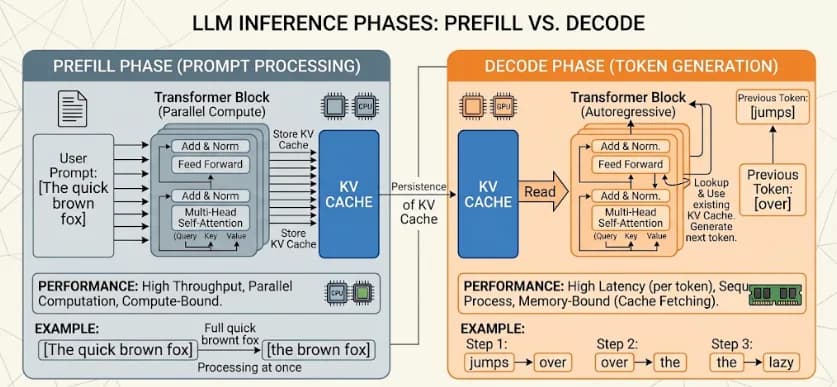
Prefill (prompt processing) is the model's first action after receiving an input. Since the entire prompt is known upfront, the model computes the hidden states for all tokens in parallel (subject to the causal mask). During this massive matrix multiplication, the model extracts and stores the key and value vectors for every prompt token, populating the initial KV cache. Because it maximizes parallel computation, prefill is typically compute-bound and dictates the Time to First Token (TTFT).
Decode (token generation) is the autoregressive loop that produces one new token at a time. At each step, the model must read the saved keys and values for all previous positions and append the newest key and value to the KV cache to generate a single token representation. Because the math is minimal but the data movement is massive, decode is highly sequential and typically memory-bandwidth-bound.
While these are the general rules, hardware specifications, batch sizes, and context lengths can shift either phase into different bottlenecks.
| Phase | Input per request | Output | Persistent effect | Bottleneck | Primary metric |
|---|---|---|---|---|---|
| Prefill | Full prompt (or chunk) | First-token logits | Populates KV cache | Compute-bound | Time to first token (TTFT) |
| Decode | One newly selected token | Next-token logits | Extends KV cache | Memory-bandwidth-bound | Inter-token latency |
When prefill and decode share the same accelerator, long prompt computations can block the rapid iteration of decode cycles. Modern serving engines mitigate this resource contention using techniques like chunked prefill (limiting how much prompt computation enters a single scheduler iteration) or disaggregated serving (assigning prefill and decode to entirely different hardware clusters and passing the KV cache state between them).
Decoding strategies
At the end of each generation step, the model produces a raw probability distribution over its vocabulary (softmax). However, the model does not actually pick the word—the decoding strategy does. A decoding strategy may always select the most likely token, sample from several likely tokens, or maintain multiple candidate sequences.
Because the chosen token is appended back to the context and permanently alters all future predictions, the decoding algorithm directly dictates the generation's diversity, quality, and computational cost.
| Strategy | Selection rule | Typical trade-off |
|---|---|---|
| Greedy | Choose the highest-probability token | Highly deterministic; optimal for extraction tasks but can become repetitive in creative text. |
| Temperature | Divide logits by a scalar before sampling | Low values sharpen focus; high values increase diversity. |
| Top-k | Sample only from the highest-probability tokens | Fixed candidate count |
| Top-p | Sample from the smallest set whose cumulative probability reaches | Candidate count adapts to uncertainty |
| Beam search | Maintain several high-scoring partial sequences | Yields high quality for constrained tasks, but heavily degrades throughput by multiplying the KV cache memory requirement by the beam width. |
Generation parameters are as critical as the model checkpoint itself. For production implementations, altering top-p or temperature can fundamentally shift both output behavior and memory utilization. See the Transformers generation guide for production implementations.
2. KV cache and attention efficiency
During causal autoregressive generation, past token representations cannot attend to future positions. Consequently, once a token's Key () and Value () vectors are computed at a given layer, their values remain completely invariant for the remainder of the sequence. Recomputing all previous keys and values at every subsequent decode step would introduce redundant compute overhead per layer.
To eliminate this redundant compute, the inference engine implements a Key-Value (KV) cache. The model computes and stores the and vectors for past positions. When generating a new token , the model only computes the Query (), Key (), and Value () projections for the newly arrived position . It appends and to the per-layer cache and performs attention by querying against the aggregated history and retrieving from .
A simplified per-layer cache tensor has the shape:
- (Batch size): The number of concurrent sequences the GPU is processing at the same time.
- (KV heads): The number of attention heads dedicated to Keys and Values. In newer models (using MQA or GQA), this is often smaller than the number of Query heads to save memory.
- (Sequence length): The cumulative context length (prompt tokens plus generated tokens).
- (Head dimension): The hidden size per individual attention head ().
While the KV cache resolves the compute bottleneck, it shifts the problem entirely to device memory (VRAM). Across all layers of a model, the total memory footprint is:
- The factor of accounts for storing two separate tensors: Keys and Values.
- is the number of transformer blocks..
- is the precision in bytes per value ( for 16-bit precision such as BF16 or FP16; for FP8).
Because KV memory scales linearly with both context length () and concurrent batch size (), it quickly dominates GPU memory capacity.
Concrete Example: Consider a 32-layer model with , , operating at 16-bit precision (). For an 8,192-token context (), a single sequence consumes:
If the serving engine processes 100 concurrent requests (), the cache alone requires over 107 GB of VRAM—surpassing the total 80 GB capacity of an NVIDIA A100 GPU before even allocating memory for the static model weights.
Where the cache physically lives?
In high-performance serving environments, model weights and the active KV cache reside directly in high-bandwidth device memory (HBM). Upon initialization, the serving runtime loads the static weights, pre-allocates execution workspaces, and assigns the remaining VRAM to a dynamic KV cache pool.
Accelerator memory (GPU HBM)
├── Model weights (static parameters)
├── Dynamic KV-cache pool
├── Short-lived activations and output logits
└── Kernel execution and graph workspaces

Host memory (CPU RAM)
├── Request queue and scheduler metadata
├── Tokenized input buffers
└── Swapped/offloaded cache blocks (evicted state)

Storage (SSD / disk)
└── Model checkpoints, tokenizer configs, quantized weight artifacts
When models exceed single-device memory limits, distributed serving partitions both the model and the KV cache:
- Tensor Parallelism (vertical split): Shards the attention heads vertically across GPUs; each worker retains the KV cache corresponding only to its assigned subset of heads ().
- Pipeline Parallelism (horizontal split): Shards the model horizontally across layers; each stage stores the KV cache only for its subset of layers ().
Managing Memory Pressure: Offloading vs. Recomputation
What happens when the VRAM pool gets full? A usual approach is offloading (swapping)-moves cache blocks to host CPU RAM. While this expands effective capacity, host memory bandwidth is substantially slower, and bus transfers introduce high latency tail spikes.
Instead of saving the cache to CPU RAM, prefix recomputation evicts cache blocks and recomputes the prefix representations on demand during future steps. This eliminates transfer overhead and frees VRAM, but trades off computational throughput.
Mitigating Cache Footprints: Grouped-Query Attention (GQA)
When an LLM generates text, it uses "Attention Heads" to look back at previous words. As we learned with the KV cache, the engine must store the Keys and Values for every single token in memory. How a model connects Queries to Keys/Values dictates how much memory it will consume.
The architectural ratio between Query heads () and Key-Value heads () directly dictates the baseline size of the KV cache.
-
Multi-Head Attention (MHA): Maximum Quality, Maximum Memory Every Query head has a dedicated Key and Value head ().The model is very smart (high "representational capacity"), but the KV cache is enormous.
-
Multi-Query Attention (MQA): Maximum Speed, Lower Quality All Query heads share a single Key head and a single Value head (). This reduces cache size by a factor of , drastically lowering memory bandwidth demand, but can degrade model expressive capacity on complex tasks.
-
Grouped-Query Attention (GQA) Serves as an optimal middle ground (). Query heads are partitioned into groups, with each group sharing one Key and Value head.
MHA (32 Q, 32 KV)       GQA (32 Q, 8 KV)            MQA (32 Q, 1 KV)
 Q Q Q Q ... Q Q        [Q Q Q Q] ... [Q Q Q Q]     [Q Q Q Q ... Q Q]
 │ │ │ │   │ │           \ /           \ /               \  /
 K K K K ... K K             K             K                 K
 V V V V ... V V             V             V                 V
 (Cache: 1.00×)             (Cache: 0.25×)           (Cache: 0.031×)
If a model has 32 query heads and 8 key-value heads, each KV pair serves 4 query heads, shrinking the cache footprint by 75% relative to standard MHA:
| Architecture | Query heads (HQ) | KV heads (HKV) | Relative KV-Cache Footprint |
|---|---|---|---|
| Multi-Head Attention (MHA) | 32 | 32 | 1.00× |
| Grouped-Query Attention (GQA) | 32 | 8 | 0.25× |
| Multi-Query Attention (MQA) | 32 | 1 | 0.03125× |
Because head counts and projection matrices () are fixed architectural parameters defined during pretraining, GQA cannot be applied purely as a post-training runtime toggle. Modern open-weight foundation models (such as LLaMA 3, Mistral, and Qwen) standardize on GQA out of the box to maximize serving efficiency.
The original GQA work showed a useful quality-speed compromise for its evaluated models: GQA: Training Generalized Multi-Query Transformer Models from Multi-Head Checkpoints.
3. FlashAttention
In standard attention, every prompt token compares itself with every token it is allowed to attend to. Mathematically, this creates an attention score matrix, where is the sequence length.
The primary bottleneck during the prefill phase is not the math itself, but the physical location where the math occurs:
- HBM (High-Bandwidth Memory): The main, large memory pool on the accelerator (e.g., an NVIDIA A100's 80 GB). It holds massive amounts of data but is relatively slow to access.
- SRAM (Static RAM): The tiny memory cache located directly on the computing chip itself. It is incredibly fast but strictly limited in size (often just 20 to 40 MB per GPU).
The Memory Wall
To execute standard attention, the GPU must materialize the entire matrix. It computes the raw scores () in SRAM, writes them out to the slow HBM, and then reads them back into SRAM to calculate the softmax probabilities (because standard softmax requires a global sum across all keys). Finally, it writes the result back to HBM. For long sequences, moving these massive intermediate matrices back and forth across the memory bus completely dominates execution time. This data traffic jam is known as the "Memory Wall."
The Solution: Tiling and Kernel Fusion
FlashAttention fundamentally changes the execution order without changing the final mathematical result. It operates via "tiling" — breaking the queries, keys, and values into small blocks that fit comfortably inside the fast SRAM.
For each query tile, FlashAttention loads the required blocks into SRAM and computes the attention scores, softmax, and value multiplication all at once. To solve the softmax problem without reading the whole row, it uses a mathematical trick called online softmax update, maintaining a running statistical tally directly in SRAM.
Because all operations are fused into a single kernel, the finished output is written back to the slow HBM only once.
Production Impact
FlashAttention is an exact, IO-aware attention algorithm, meaning it produces the exact same result as standard attention (subject only to standard floating-point variance). It is important to note what it does and does not do:
- It does not remove the arithmetic computations (FLOPs), shrink the model weights, or reduce the persistent memory footprint of the decode KV cache.
- It does drastically reduce memory traffic and eliminate the need to allocate HBM for the temporary attention matrix.
Production serving engines invoke highly optimized, hardware-specific implementations of this algorithm rather than recreating it in application code. By completely eliminating the intermediate memory overhead, FlashAttention is the primary engineering breakthrough that allows modern LLMs to process massive context windows (like entire books or codebases) without suffering catastrophic out-of-memory (OOM) errors.
The method is described in FlashAttention: Fast and Memory-Efficient Exact Attention with IO-Awareness.
4. PagedAttention and vLLM
The Fragmentation Problem
Naive inference engines allocate a contiguous chunk of GPU memory based on a request's maximum possible sequence length. Because most requests finish long before reaching this maximum limit, huge portions of the reserved memory remain completely empty. This wasted space is called "fragmentation." Furthermore, as these large contiguous blocks are allocated and freed, the remaining free memory becomes Swiss cheese (external fragmentation)—preventing the system from accepting new requests even when total available VRAM is theoretically sufficient.
PagedAttention solves this bottleneck by borrowing a foundational concept from computer operating systems: virtual memory paging.
Instead of reserving one massive, contiguous chunk of memory per request, PagedAttention divides the KV cache into small, fixed-size physical blocks (e.g., storing the vectors for 16 or 32 tokens). Each sequence is assigned a logical block table whose entries point to these physical blocks scattered across a shared memory pool.
Request A: logical [0] [1] [2] ──► physical [7] [2] [11]
Request B: logical [0] [1]     ──► physical [4] [9]
Free pool:                           [1] [3] [5] [6] [8] [10] ...
When a request starts the prefill phase, it is only allocated the exact number of blocks it needs. As the model generates text during the decode phase, the system dynamically provisions one new physical block at a time. Because the attention kernel knows how to read the block table map, the physical memory can be scattered randomly across the GPU without issue.
Blocks are allocated strictly as sequences grow and returned immediately when requests finish, meaning waste is limited strictly to the final, partially filled block.
Prefix Sharing and vLLM
Because memory is mapped logically, PagedAttention enables Copy-on-Write (CoW) memory sharing via reference counting. If multiple requests share the exact same system prompt, or if a generation strategy like beam search branches out from a single prefix, the sequences can safely point to the exact same physical blocks for the shared context, saving massive amounts of memory. (Note: These “pages” are a software-level cache abstraction managed by the inference engine, not literal hardware OS pages).
The open-source serving engine vLLM pioneered this technique, pairing paged cache management with a continuous batching scheduler. While PagedAttention maximizes usable cache capacity, the scheduler weaponizes that freed capacity to massively increase concurrent throughput.
For implementation specifics, see Efficient Memory Management for Large Language Model Serving with PagedAttention.
Operational Debugging: Choosing the Right Optimization
Attention and cache optimizations should not be applied blindly; they must be chosen based on measured constraints in the production environment.
| Observed symptom | Likely pressure | Candidate interventions |
|---|---|---|
| High TTFT for long prompts | Prefill compute, attention IO, or scheduling queue | FlashAttention, chunked prefill, prefix caching, prompt truncation, or disaggregated prefill serving. |
| KV-cache OOM or low concurrency | Cache capacity or fragmentation limits | PagedAttention, migrating to a model with GQA/MQA, KV-cache quantization (e.g., FP8), or adding device memory. |
To summarize the stack: FlashAttention accelerates the physical execution of attention math, GQA permanently shrinks the baseline architectural shape of the cache, and PagedAttention dynamically manages how that cache is allocated in real-time. They are entirely complementary, but none substitutes for strictly monitoring the actual serving workload.
5. Breaking the bandwidth bottleneck: model compression
In addition to managing VRAM capacity and attention IO, engineers can optimize the payload itself to circumvent the strict autoregressive bottleneck. There are several architectural and mathematical techniques to make massive LLMs smaller, faster, and more efficient to serve.
Number formats
Number formats dictate a model's memory footprint, dynamic range, and which hardware kernels are invoked during execution.
| Format | Bits | Bytes/Value | Characteristics |
|---|---|---|---|
| FP32 | 32 | 4.0 | Maximum range and precision; strictly computationally prohibitive for LLM inference. |
| FP16 | 16 | 2.0 | Standard inference format; high fractional precision but smaller dynamic range than BF16. |
| BF16 | 16 | 2.0 | FP32-like exponent range with fewer fractional bits; highly stable. |
| INT8 | 8 | 1.0 | Halves memory footprint; requires scaling metadata to reconstruct values. |
| INT4 | 4 | 0.5 | Highly compressed; packs two values per byte before scales and metadata. |
Storage precision and computation precision are not always identical. In Weight-Only Quantization (WOQ), a GPU stores the model weights in INT4 to drastically reduce VRAM footprint and memory bandwidth demands. The compression is mostly to solve the data-movement bottleneck (the Memory Wall). However, during execution, the kernel unpacks those INT4 values back into FP16 to perform the actual matrix multiplication.
Quantisation
Quantization is the mathematical process of mapping high-resolution floating-point numbers (FP16) into low-resolution integer spaces (INT8/INT4).
A standard symmetric quantization scheme operates by calculating a scale factor () and clamping the rounded values:
To utilize the tensor during inference, the kernel multiplies it by the scale to reconstruct an approximation (). Conceptually, it divides the tensor's dynamic range into discrete buckets, forces every number into its nearest bucket, and stores only the bucket ID.
The scale reconstructs an approximation . Practical LLM quantisers typically use per-channel or grouped scales, clipping, outlier handling, and packed kernels.
When implementing quantization, several critical distinctions arise:
- Weight-only vs. Weight-and-Activation: Compressing only weights targets the memory bandwidth wall. Compressing activations alongside weights enables specialized, high-throughput integer compute kernels (like INT8 Tensor Cores) but is highly sensitive to outlier values.
- Post-training Quantisation (PTQ) vs. Quantisation-aware Training (QAT): PTQ mathematically compresses a frozen checkpoint; QAT simulates these precision drops during the pretraining phase, allowing the network to adapt to the information loss.
- Component Isolation: The static model weights and the dynamic KV cache exist as separate memory pools and can safely utilize entirely different quantization formats (e.g., FP4 weights with an FP8 KV cache).
Because compression alters the fundamental precision of the model, fewer bits do not automatically guarantee lower latency unless the target hardware possesses an optimized execution kernel for that specific format. Furthermore, aggressive quantization can introduce silent quality regressions. Evaluation must go beyond basic memory profiling to include task accuracy, perplexity, structured-output validity, TTFT, and inter-token latency (ITL) under representative loads. The Hugging Face quantisation documentation summarizes supported production integrations such as AWQ, GPTQ, and bitsandbytes.
If compression produces a quality regression, the correct operational response is rarely more serving optimization. Instead, engineers must revisit the calibration data, adjust the quantization group size, retain highly sensitive layers at a higher precision, or simply restore the previous format. Performance changes must pass the exact same task-level and safety evaluations as an entirely new model release.
Knowledge distillation
While quantization mathematically compresses an existing model, knowledge distillation is a pre-deployment training technique that forces a smaller "student" model to imitate a massive "teacher" model.
Standard pretraining relies on hard targets (e.g., next-token prediction). If the prompt is "The dog chased the...", the dataset simply dictates the answer is "cat". In distillation, the teacher model exposes its entire predicted probability distribution: "I am 80% sure it is 'cat', but 15% sure it is 'squirrel', and 5% sure it is 'ball'."
By calculating the cross-entropy alongside the KL divergence between these softened distributions, the student learns nuanced relationships and generalized logic that it could never infer from hard labels alone:
The resulting student model requires less VRAM, features a smaller hidden width, and generates tokens faster—acting as a permanent architectural optimization before inference even begins.
The foundational method is described in Distilling the Knowledge in a Neural Network.
Speculative decoding
Distillation replaces the large model with a student. Speculative decoding explicitly targets the memory bandwidth wall by trading spare computational power for reduced VRAM reads.
Speculative decoding keeps the target model and uses a cheaper draft process (a tiny, cheap model) to propose multiple tokens. The target scores those proposed positions in one parallel pass and accepts a prefix of them.
Draft (Small Model):   Rapidly proposes candidate sequence [t1, t2, t3, t4]
Target (Large Model):  Verifies all proposed positions simultaneously
Result:                Accepts the valid prefix; corrects upon rejection
Because the target model evaluates the entire drafted sequence in a single forward pass, it only has to read its massive weight matrices from HBM once. For exact sampling, a token proposed from draft distribution is accepted with a probability of .
If the lightweight draft model predicts accurately, the system successfully generates multiple tokens for the IO cost of a single memory read. If it fails, the target model rejects the sequence, corrects the prediction, and seamlessly resumes the autoregressive loop.
See Fast Inference from Transformers via Speculative Decoding.
6. From inference mechanics to a service
The mathematical realities of the KV cache represent the fundamental bridge between model execution and serving capacity. Its VRAM footprint dictates exactly how many concurrent sequences can physically fit onto a GPU; its autoregressive growth forces request scheduling to be dynamic; and the extreme hardware differences between the compute-heavy prefill and the memory-bound decode phases dictate our core performance metrics: Time to First Token (TTFT) and Inter-Token Latency (ITL).
By combining memory management frameworks like PagedAttention with model compression strategies like quantization and speculative decoding, we can fundamentally alter the execution math to survive these hardware bottlenecks.
The final article in this series, Running LLMs in Production: Batching, Quantization, and Service-Level Objectives, takes these optimized inference mechanics and turns them into a production reality. We will explore how serving engines handle continuous request queues, distribute workloads across different GPU clusters, enforce Service-Level Objectives (SLOs), and monitor system performance.
本文是三部曲的第二篇。第一篇〈LLM 預訓練:深入解析純解碼器 Transformer〉說明了模型如何將原始文字轉換為下一個 token 的機率分布。
預訓練只是起點。訓練完成、模型權重固定後,挑戰的重心便從「學習」轉向「執行」。在正式環境中,提示詞會動態抵達,每個新生成的 token 都會加入既有上下文,使注意力狀態持續增長。每項請求不僅要依序生成 token,還要維護各自的狀態;因此,核心問題也從訓練運算轉變為記憶體頻寬、硬體利用率與動態狀態管理。
| 面向 | 預訓練 | 推論 |
|---|---|---|
| 輸入 | 大批次、完整的序列 | 隨時間動態抵達的提示詞 |
| 目標 | 最小化下一個 token 的損失 | 在記憶體與延遲限制內生成有用的 token |
| 狀態 | 權重、梯度、最佳化器狀態、激活值 | 權重,以及每個請求各自的 KV 快取 |
| 平行化 | 大量序列位置同時處理 | 預填充可平行處理;解碼則以自迴歸方式逐步進行 |
| 記憶體壓力 | 參數、梯度、優化器、激活值 | 參數、KV 快取、硬體工作空間 |
| 主要指標 | 每秒訓練 token 數、收斂情況、使用率 | 首個 token 生成時間(TTFT)、token 間延遲、吞吐量 |
(更完整的服務架構、請求排程與服務等級目標,將在本系列的最終篇中說明。)
本文將說明 LLM 推論為何帶來與訓練截然不同的系統挑戰,以及 KV 快取、FlashAttention、PagedAttention 與模型壓縮如何管理持續增長的注意力狀態、緩解頻寬瓶頸,並提升整體執行效率。
本文結構如下:
1. 推論的兩個階段:預填充與解碼
當一個大型語言模型生成回應時,其前向傳播會被拆分成兩個截然不同的階段,各自有著完全不同的硬體瓶頸與效能特性。
預填充(Prefill),也就是提示詞處理,是模型收到輸入後的第一個階段。由於完整提示詞已知,模型可以在因果遮罩的限制下,平行計算所有 token 的隱藏狀態。在大量矩陣乘法的過程中,模型會為提示詞中的每個 token 計算並儲存 Key 與 Value 向量,建立初始 KV 快取。預填充通常較偏向計算受限,並直接影響首個 token 生成時間(TTFT)。
解碼(Decode),也就是 token 生成,是每次產生一個新 token 的自迴歸迴圈。每一步都要讀取先前位置已儲存的 Key 與 Value,再將最新的 Key 與 Value 加入 KV 快取。相較於需要搬移的權重與快取資料,單步解碼的運算量通常較小,因此這個階段往往受記憶體頻寬限制,且無法跨生成步驟完全平行化。
雖然這是一般通則,但硬體規格、批次大小與上下文長度,都可能讓任一階段的瓶頸發生轉移。
| 階段 | 每個請求的輸入 | 輸出 | 持續性影響 | 瓶頸 | 主要指標 |
|---|---|---|---|---|---|
| 預填充 | 完整提示詞(或其中一塊) | 第一個 token 的 logits | 填入 KV 快取 | 計算受限 | 首個 token 生成時間(TTFT) |
| 解碼 | 一個新選出的 token | 下一個 token 的 logits | 擴充 KV 快取 | 記憶體頻寬受限 | token 間延遲 |
當預填充與解碼共用同一個加速器時,冗長提示詞的運算可能會阻塞解碼週期的快速迭代。現代服務引擎會透過分塊預填充(限制單一排程週期內能處理多少提示詞運算)或分離式服務(disaggregated serving,將預填充與解碼分派給完全不同的硬體叢集,並在兩者之間傳遞 KV 快取狀態)等技術,來緩解這種資源爭用。
解碼策略
每個生成步驟結束時,模型會輸出涵蓋整個詞彙表的 logits,再經 softmax 轉換為機率分布。不過,機率分布本身不會決定唯一輸出;系統仍需要解碼策略,才能選出實際要加入序列的 token。它可以直接選擇機率最高者、從高機率候選中採樣,或同時維護多條候選序列。
由於選定的 token 會被附加回上下文,並永久改變之後所有的預測,解碼演算法直接決定了生成結果的多樣性、品質與運算成本。
| 策略 | 選擇規則 | 典型的取捨 |
|---|---|---|
| 貪婪解碼 | 選擇機率最高的 token | 高度確定性;適合擷取類任務,但在創意文本中容易變得重複。 |
| 溫度採樣 | 採樣前先將 logits 除以一個純量 | 數值越低越聚焦;數值越高越多樣。 |
| Top-k | 僅從機率最高的 個 token 中採樣 | 候選數量固定 |
| Top-p | 從累積機率達到 的最小集合中採樣 | 候選數量會依不確定性自動調整 |
| 集束搜尋(Beam search) | 同時維護多條高分的部分序列 | 對限制性任務能產生高品質結果,但會讓 KV 快取的記憶體需求乘上集束寬度,大幅拉低吞吐量。 |
生成參數是模型版本之外的重要設定。調整 top-p、溫度或 beam width,可能明顯改變輸出行為、延遲與記憶體需求。實作方式可參考 Transformers 生成指南。
2. KV 快取與注意力效率
在因果自迴歸生成的過程中,過去 token 的表示無法關注到未來的位置。因此,一旦某個 token 在某一層的 Key()與 Value()向量計算完成,這些數值在序列剩餘的部分中,就會保持完全不變。若每一次後續的解碼步驟,都要重新計算所有先前的 key 與 value,每一層都會產生 的多餘運算成本。
為了消除這種多餘的運算,推論引擎會實作一個 Key-Value(KV)快取。模型會計算並儲存過去各個位置的 與 向量。在生成新的 token 時,模型只需計算新抵達位置 的 Query()、Key()與 Value()投影。它會將 與 附加到每一層各自的快取中,並透過拿 與累積的歷史 做比對、再從 中取值,來執行注意力運算。
簡化後,每一層的快取張量形狀為:
- (批次大小):GPU 同時處理的並發序列數量。
- (KV head 數):專門用於 Key 與 Value 的注意力 head 數量。在較新的模型中(採用 MQA 或 GQA),這個數字通常會小於 Query head 的數量,藉此節省記憶體。
- (序列長度):累積的上下文長度(提示詞 token 加上已生成的 token)。
- (head 維度):每個注意力 head 各自的隱藏維度大小()。
KV 快取避免了重複計算,代價則是增加裝置記憶體(VRAM)用量。涵蓋模型全部 層時,總記憶體用量為:
- 這裡的係數 ,代表要儲存兩個獨立的張量:Key 與 Value。
- 是 transformer block 的數量。
- 是每個數值所佔的位元組數(16 位元精度,例如 BF16 或 FP16,;FP8 則 )。
由於 KV 快取用量會隨上下文長度()與同時處理的序列數()線性成長,它很快就可能成為 GPU 記憶體容量的主要限制。
具體範例:假設有一個 32 層的模型,,,以 16 位元精度運作()。對於一個 8,192 token 的上下文(),單一序列會消耗:
如果服務引擎同時處理 100 個並發請求(),光是快取就需要超過 107 GB 的 VRAM——這已經超過一張 NVIDIA A100 GPU 總共 80 GB 的容量,而這還不包括靜態模型權重所需要的記憶體。
快取實際存放在哪裡?
在高效能的服務環境中,模型權重與運作中的 KV 快取,會直接存放在高頻寬裝置記憶體(HBM)中。初始化時,服務執行環境會載入靜態權重、預先配置執行用的工作空間,並將剩餘的 VRAM 分配給動態的 KV 快取池。
加速器記憶體(GPU HBM)
├── 模型權重(靜態參數)
├── 動態 KV 快取池
├── 短暫存在的激活值與輸出 logits
└── Kernel 執行與計算圖工作空間

主機記憶體(CPU RAM)
├── 請求佇列與排程器中繼資料
├── 已 tokenize 的輸入緩衝區
└── 已置換/卸載的快取區塊(已驅逐的狀態)

儲存空間(SSD/磁碟)
└── 模型檢查點、tokenizer 設定、量化後的權重檔案
當模型超出單一裝置的記憶體限制時,分散式服務會同時將模型與 KV 快取切分:
- 張量平行(垂直切分):將注意力 head 垂直切分到多張 GPU 上;每個工作節點,只保留自己被分配到那部分 head 所對應的 KV 快取()。
- 管線平行(水平切分):將模型依層水平切分;每個階段,只儲存自己那部分層所對應的 KV 快取()。
管理記憶體壓力:卸載 vs. 重新計算
當 VRAM 池被用滿時,會發生什麼事?常見的做法是卸載(swapping,置換)——把快取區塊搬到主機的 CPU RAM。雖然這能擴大有效容量,但主機記憶體的頻寬慢得多,匯流排傳輸也會導致嚴重的延遲尾端尖峰。
與其把快取存到 CPU RAM,前綴重新計算則是直接驅逐快取區塊,在之後的步驟中,按需重新計算前綴的表示。這樣能省去傳輸開銷、釋放 VRAM,但代價是犧牲運算吞吐量。
縮減快取用量:分組查詢注意力(GQA)
當 LLM 生成文字時,會用「注意力 head」回頭查看先前的詞語。正如我們在 KV 快取中所學到的,引擎必須在記憶體中儲存每一個 token 的 Key 與 Value。模型將 Query 連結到 Key/Value 的方式,直接決定了會消耗多少記憶體。
Query head()與 Key-Value head()之間的架構比例,直接決定了 KV 快取的基準大小。
-
多頭注意力(MHA):每個 Query head 都有專屬的 Key 與 Value head(),保留完整的多頭表示能力,但 KV 快取用量最大。
-
多查詢注意力(MQA):所有 Query head 共用單一 Key head 與單一 Value head()。這會把快取大小縮減為 MHA 的 ,並大幅降低記憶體頻寬需求,但部分模型或任務可能面臨品質取捨。
-
分組查詢注意力(GQA):是介於兩者之間的常見實務折衷()。Query head 會分成多組,每組共用一個 Key 與 Value head。
MHA(32 個 Q,32 個 KV)  GQA(32 個 Q,8 個 KV)      MQA(32 個 Q,1 個 KV)
 Q Q Q Q ... Q Q        [Q Q Q Q] ... [Q Q Q Q]     [Q Q Q Q ... Q Q]
 │ │ │ │   │ │           \ /           \ /               \  /
 K K K K ... K K             K             K                 K
 V V V V ... V V             V             V                 V
 (快取:1.00×)             (快取:0.25×)           (快取:0.031×)
如果一個模型有 32 個 query head 與 8 個 key-value head,那麼每一組 KV 就會服務 4 個 query head,相較於標準 MHA,快取用量會縮減 75%:
| 架構 | Query head 數() | KV head 數() | 相對 KV 快取用量 |
|---|---|---|---|
| 多頭注意力(MHA) | 32 | 32 | 1.00× |
| 分組查詢注意力(GQA) | 32 | 8 | 0.25× |
| 多查詢注意力(MQA) | 32 | 1 | 0.03125× |
由於 head 數量與投影矩陣()是在訓練前就決定的架構參數,GQA 不能在模型完成訓練後,單純透過執行期開關啟用。許多現代開放權重基礎模型(例如 Llama 3、Mistral、Qwen)預設採用 GQA,以兼顧模型能力與服務效率。
GQA 的原始論文,針對其評估的模型,展示了一種實用的品質與速度折衷方案:〈GQA: Training Generalized Multi-Query Transformer Models from Multi-Head Checkpoints〉。
3. FlashAttention
在標準注意力機制中,提示詞裡的每一個 token,都會與它被允許關注的每一個 token 相互比較。從數學上看,這會產生一個 的注意力分數矩陣,其中 是序列長度。
預填充階段的效能不只取決於算術運算量,也取決於資料在不同層級記憶體之間的搬移方式:
- HBM(高頻寬記憶體):加速器上的主要記憶體,容量較大,負責存放模型權重、KV 快取與張量資料;相較於晶片內記憶體,存取延遲與資料搬移成本較高。
- SRAM(靜態隨機存取記憶體):位於運算晶片內的高速記憶體,存取速度快,但容量有限。
記憶體牆
要執行標準的注意力運算,GPU 必須實際生成整個 矩陣。它會先在 SRAM 中計算原始分數(),將結果寫出到速度較慢的 HBM,接著再讀回 SRAM 以計算 softmax 機率(因為標準 softmax 需要對所有 key 做全域加總)。最後,再把結果寫回 HBM。對於長序列而言,這些龐大的中間矩陣,在記憶體匯流排上來回搬移所耗費的時間,會完全主宰整個執行時間。這種資料交通壅塞,就稱為「記憶體牆」。
解決方案:分塊與 Kernel 融合
FlashAttention 重新安排注意力運算的執行順序,但不改變其數學定義。它採用**分塊(tiling)**技術,將 Query、Key 與 Value 拆成能完整放入高速 SRAM 的小區塊。
對於每一個 query 區塊,FlashAttention 會把所需的區塊載入 SRAM,一次性計算出注意力分數、softmax 與 value 相乘的結果。為了在不讀取整列資料的情況下解決 softmax 的問題,它使用了一種稱為線上 softmax 更新的數學技巧,直接在 SRAM 中維護一份持續更新的統計數值。
由於所有運算都被融合成單一一個 kernel,完成後的輸出只需要寫回速度較慢的 HBM 一次。
對正式環境的影響
FlashAttention 是一個精確、具備 IO 感知能力的注意力演算法,意味著它產生的結果,與標準注意力完全相同(僅受一般浮點數運算誤差影響)。有件事值得特別留意,它做到了什麼、又沒做到什麼:
- 它不會移除 的算術運算量(FLOPs)、不會縮小模型權重,也不會減少解碼階段 KV 快取的持續性記憶體用量。
- 它確實會大幅減少記憶體流量,並免除為暫存的 注意力矩陣配置 HBM 空間的需求。
正式環境的服務引擎通常會呼叫針對特定硬體最佳化的實作,而不是在應用程式碼中自行重寫。FlashAttention 大幅減少中間張量的記憶體流量與空間需求,因此是支援長上下文的重要技術之一;不過,可處理的實際長度仍受模型設定、KV 快取與裝置容量限制。
此方法記載於〈FlashAttention: Fast and Memory-Efficient Exact Attention with IO-Awareness〉。
4. PagedAttention 與 vLLM
記憶體碎片化問題
簡單的推論引擎可能依照請求可達到的最大序列長度,預先配置一整塊連續 GPU 記憶體。然而,多數請求會在達到上限前結束,使部分保留空間始終未被使用,形成內部碎片。另一方面,大型連續區塊反覆配置與釋放後,可用空間可能分散在不同位置,形成外部碎片;即使剩餘 VRAM 的總量足夠,也未必能配置新的大型連續區塊。
PagedAttention 借用了電腦作業系統中的一項基礎概念——虛擬記憶體分頁機制,來解決這個瓶頸。
PagedAttention 不會為每個請求保留一整塊龐大的連續記憶體,而是把 KV 快取切分成一個個固定大小的小型實體區塊(例如,每個區塊儲存 16 或 32 個 token 的向量)。每個序列,都會被分配一份邏輯區塊表,表中的每個項目,都指向散布在共享記憶體池中的這些實體區塊。
請求 A:邏輯 [0] [1] [2] ──► 實體 [7] [2] [11]
請求 B:邏輯 [0] [1]     ──► 實體 [4] [9]
空閒池:                     [1] [3] [5] [6] [8] [10] ...
請求進入預填充階段時,系統只配置當下所需的區塊;進入解碼階段後,再隨序列增長動態配置新的實體區塊。注意力 kernel 會根據區塊表定位資料,因此各區塊不必在實體記憶體中連續排列。
區塊會嚴格依照序列的成長逐步配置,並在請求結束時立即歸還,這意味著浪費的空間,就只會限於最後那個未填滿的區塊。
前綴共享與 vLLM
由於記憶體是以邏輯方式對應的,PagedAttention 能透過參照計數,實現寫入時複製(Copy-on-Write,CoW)的記憶體共享。如果多個請求共用完全相同的系統提示詞,或是像集束搜尋這樣的生成策略,從單一前綴分岔出多條路徑,這些序列就能安全地指向完全相同的實體區塊來存放共用的上下文,藉此節省大量記憶體。(附註:這裡的「頁」,是推論引擎所管理的軟體層級快取抽象概念,並不是真正的硬體作業系統分頁。)
開源服務引擎 vLLM 推廣了這項技術,並將分頁式快取管理與連續批次排程結合。PagedAttention 提升 KV 快取空間的使用效率,排程器則利用可用容量容納更多進行中的序列,進而改善並行度與吞吐量。
實作細節請參見〈Efficient Memory Management for Large Language Model Serving with PagedAttention〉。
實務除錯:選擇正確的優化方式
注意力與快取相關的最佳化必須根據正式環境中實際量測到的瓶頸選擇,而不是一律套用。
| 觀察到的症狀 | 可能的壓力來源 | 可能的介入方式 |
|---|---|---|
| 長提示詞的 TTFT 偏高 | 預填充運算量、注意力 IO,或排程佇列 | FlashAttention、分塊預填充、前綴快取、提示詞截斷,或分離式預填充服務。 |
| KV 快取記憶體不足或並發數過低 | 快取容量或碎片化限制 | PagedAttention、改用具備 GQA/MQA 的模型、KV 快取量化(例如 FP8),或增加裝置記憶體。 |
總結來說,FlashAttention 改善注意力運算的記憶體存取效率,GQA 從模型架構層面縮小 KV 快取的基準大小,PagedAttention 則動態管理快取配置。三者處理的是不同層次的問題,彼此可以互補,但仍不能取代對實際服務負載的持續監控。
5. 打破頻寬瓶頸:模型壓縮
除了管理 VRAM 容量與注意力 IO 之外,工程師還能直接優化承載的內容本身,藉此繞過嚴格的自迴歸瓶頸。有好幾種架構與數學層面的技術,能讓龐大的 LLM 變得更小、更快,也更有效率地提供服務。
數值格式
數值格式決定了模型的記憶體用量、動態範圍,以及執行時會呼叫哪些硬體 kernel。
| 格式 | 位元數 | 每個數值的位元組數 | 特性 |
|---|---|---|---|
| FP32 | 32 | 4.0 | 精度高、動態範圍大,但用於大規模 LLM 推論時,記憶體與頻寬成本通常較高。 |
| FP16 | 16 | 2.0 | 標準推論格式;小數精度高,但動態範圍比 BF16 小。 |
| BF16 | 16 | 2.0 | 指數範圍與 FP32 相近,但小數位元較少;穩定性高。 |
| INT8 | 8 | 1.0 | 記憶體用量減半;需要縮放中繼資料才能還原數值。 |
| INT4 | 4 | 0.5 | 高度壓縮;在加入縮放與中繼資料之前,每個位元組可打包兩個數值。 |
儲存精度與運算精度,並不總是一致的。在純權重量化(Weight-Only Quantization,WOQ)中,GPU 會以 INT4 格式儲存模型權重,藉此大幅降低 VRAM 用量與記憶體頻寬需求。這種壓縮,主要是為了解決資料搬移的瓶頸(也就是記憶體牆)。然而,在實際執行時,kernel 會把這些 INT4 數值解包回 FP16,才能進行真正的矩陣乘法運算。
量化
量化是將較高精度的數值表示(例如 FP16)映射到較低位元格式(例如 INT8 或 INT4)的過程。
標準的對稱量化方案,運作方式是計算出一個縮放因子(),再將四捨五入後的數值做截斷:
在推論時要使用這個張量,kernel 會將它乘上縮放因子,還原出一個近似值()。從概念上來說,這個做法把張量的動態範圍切分成一個個離散的「桶」,強制把每個數值歸入最接近的桶,並只儲存桶的編號。
縮放因子 會用來還原出近似值 。實務上的 LLM 量化器,通常會採用逐通道或分組的縮放係數、裁剪、離群值處理,以及打包後的 kernel。
在實作量化時,有幾個關鍵的區別需要留意:
- 純權重量化 vs. 權重與激活值量化: 只壓縮權重,鎖定的是記憶體頻寬這道牆。同時壓縮激活值與權重,能啟用專門、高吞吐量的整數運算 kernel(例如 INT8 Tensor Core),但對離群值非常敏感。
- 訓練後量化(PTQ)vs. 量化感知訓練(QAT): PTQ 直接量化已完成訓練的模型;QAT 則在訓練或再訓練過程中模擬低精度運算,讓模型適應量化誤差。
- 元件分開處理: 靜態模型權重與動態 KV 快取是不同的記憶體區域,可以採用不同的量化格式(例如權重使用 FP4、KV 快取使用 FP8),但都必須分別驗證硬體支援與品質影響。
由於壓縮會改變模型的基礎精度,除非目標硬體針對該特定格式有優化過的執行 kernel,否則位元數變少,並不會自動保證延遲降低。此外,過於激進的量化,可能會引入不易察覺的品質衰退。評估工作不能只停留在基本的記憶體分析,還必須涵蓋任務準確度、困惑度、結構化輸出的有效性,以及在具代表性負載下的 TTFT 與 token 間延遲(ITL)。Hugging Face 的量化文件,整理了正式環境中受支援的整合方案,例如 AWQ、GPTQ 與 bitsandbytes。
如果壓縮導致品質下降,應先重新檢視校準資料、量化分組大小與各層的敏感度,必要時讓部分層保留較高精度,或恢復原先格式。任何效能調整都應接受與新模型版本相同的任務品質與安全性評估。
知識蒸餾
量化是對既有模型進行數學上的壓縮,而知識蒸餾則是一種部署前的訓練技術,讓一個較小的「學生」模型,去模仿一個龐大的「教師」模型。
標準的預訓練,仰賴的是硬性目標(例如下一個 token 預測)。如果提示詞是「The dog chased the...」,資料集就只會直接規定答案是「cat」。而在蒸餾中,教師模型會揭露它完整的預測機率分布:「我有 80% 的把握是『cat』,但也有 15% 的把握是『squirrel』,5% 的把握是『ball』。」
透過結合硬標籤的交叉熵與教師、學生機率分布之間的 KL 散度,學生模型能取得比單一正確答案更豐富的類別關係訊號:
最終得到的學生模型通常參數較少、VRAM 需求較低,也可能具備更快的 token 生成速度。這是在部署前透過訓練完成的模型壓縮,而不是推論期間才啟用的執行技巧。
此基礎方法記載於〈Distilling the Knowledge in a Neural Network〉。
推測解碼
蒸餾以較小的學生模型取代原模型;推測解碼則保留目標模型,利用額外運算換取較少的序列化解碼步驟。
推測解碼會保留目標模型,並使用成本較低的草稿流程(一個微小、便宜的模型)來提議多個 token。目標模型接著會在一次平行的前向傳播中,為這些被提議的位置打分,並接受其中的一段前綴。
草稿模型(小模型):     快速提議候選序列 [t1, t2, t3, t4]
目標模型(大模型):     同時驗證所有被提議的位置
結果:                有效的前綴會被接受;遭拒絕的部分則會被修正
由於目標模型是在單一一次前向傳播中,評估整段草稿序列,它只需要從 HBM 讀取一次龐大的權重矩陣。若要做到精確採樣,從草稿分布 中提議出的 token ,會以 的機率被接受。
如果輕量草稿模型的提議具有足夠高的接受率,目標模型便可能在一次驗證中接受多個 token,降低逐 token 執行目標模型的次數。若部分提議遭到拒絕,演算法會依規則修正輸出,再繼續自迴歸生成。
詳見〈Fast Inference from Transformers via Speculative Decoding〉。
6. 從推論機制到正式服務
KV 快取是連結模型執行與服務容量的核心狀態。它的 VRAM 用量會影響單張 GPU 可容納的同時序列數;它隨序列增長的特性要求排程器動態管理資源;而預填充與解碼的不同硬體瓶頸,則分別影響首個 token 生成時間(TTFT)與 token 間延遲(ITL)。
結合 PagedAttention 等記憶體管理技術,以及量化、推測解碼等方法,可以從不同層面改善容量、頻寬與延遲瓶頸。實際效果仍必須在具代表性的服務負載與品質要求下量測。
本系列的最後一篇文章〈在正式環境中運行 LLM:批次處理、量化與服務等級目標〉,會將這些經過優化的推論機制,轉化成正式環境中的現實。我們會探討服務引擎如何處理連續不斷的請求佇列、如何在不同的 GPU 叢集之間分配工作負載、如何落實服務等級目標(SLO),以及如何監控系統效能。