LLM Serving: Continuous Batching, Distributed Execution, and Service-Level ObjectivesLLM 正式環境部署:批次處理、分散式推論與服務等級目標
How do you serve 10,000 concurrent users? A deep dive into continuous batching, disaggregated prefill architectures, and multi-GPU parallelism to meet strict Service-Level Objectives in production, plus a troubleshooting quick-reference.深入解析連續批次處理、分離式預填充、多 GPU 平行化與 SLO,說明如何將模型檢查點轉化為可擴展、可監控的正式服務。
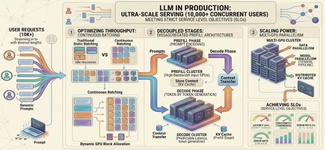
This is the final article in a three-part series. The first article deconstructed the mathematical anatomy of a decoder-only transformer. The second article zoomed in on hardware execution, exploring how KV caching, FlashAttention, and model compression tame the strict memory-bandwidth bottlenecks of the generation loop. This article focuses on running LLMs in the production system.
But a highly optimized model is only half the battle. In a vacuum, generating tokens is an algorithmic challenge; in production, it is a distributed systems challenge.
This final article steps outside the model's architecture. We focus on the infrastructure required to turn a raw computational graph into a scalable, highly concurrent service. We will explore how to dynamically schedule continuous request queues, distribute massive models across multi-GPU clusters, and navigate the unavoidable tension between throughput, latency, and hardware costs to guarantee strict Service-Level Objectives (SLOs).
The content is structured as:
- Request orchestration: Batching strategies
- Scaling execution: Model parallelism
- The core tension: Throughput, latency, and cost
- SLO thinking and serving frameworks
- Infrastructure and system design reference
- Conclusion
1. Request orchestration: Batching strategies
Unlike traditional microservices where inputs are uniform (predictable data types or fixed-schema JSON payloads), LLM inference workloads are highly heterogeneous:
- Asynchronous arrival: Users and automated systems send prompts at entirely unpredictable intervals.
- Variable lengths: One request might be a five-token classification prompt, while the next requires processing a 10,000-token document.
If a GPU processes these requests sequentially, it sits mostly idle, starved for compute. To maximize hardware utilization, serving engines group multiple requests into batches. However, because requests do not finish at the same time, how the engine forms these batches dictates the system's performance.
The Evolution of Batching
In production, a batch usually contains independent requests from multiple users. Batching never mixes the actual text of different users; it simply groups their independent tensor operations for parallel execution on the accelerator, with each request maintaining its own sequence state, decoding parameters, and KV cache.
| Strategy | Mechanism | Production Limitation |
|---|---|---|
| Static batching | The server waits for a predefined number of requests, pads them to the length of the longest prompt, and executes them together. | Severe latency degradation; short sequences remain trapped waiting for long sequences to finish. |
| Dynamic batching | The server opens a brief time window (e.g., 50ms) to collect incoming requests into a batch before execution. | Improved throughput, but batch membership still only changes at request boundaries. |
| Continuous batching | The scheduler operates strictly at the token level. It ejects finished sequences and pulls new requests into the active batch at every single iteration step. | Requires advanced cache-aware memory management (like PagedAttention) to function. |
Continuous batching (iteration-level scheduling) is the modern industry standard. Because finished sequences leave immediately and waiting requests take their place in the very next decode step, GPU downtime drops to nearly zero. This is the key throughput innovation in vLLM and TGI. GPU utilization goes from ~40-60% (static) to ~90%+ (continuous).
Time (Iteration Steps) ──────────────────────────────────────►

Step 1: [ Req 1 | Req 2 | Req 3 | Req 4 ]
Step 2: [ Req 1 | Req 2 | Req 3 | Req 5 ]  ← Req 4 finishes, Req 5 enters instantly
Step 3: [ Req 1 | Req 6 | Req 3 | Req 5 ]  ← Req 2 finishes, Req 6 enters instantly
Step 4: [ Req 1 | Req 6 | Req 7 | Req 5 ]  ← Req 3 finishes, Req 7 enters instantly

Result: Zero wait time at request boundaries. The GPU is always fully utilized.
Advanced Scheduling Policies
Beyond the core batching loop, schedulers must balance fairness, priority, and physical memory limits using advanced policies.
Handling Memory Exhaustion: Preemption
If active requests generate longer responses than anticipated and the GPU's KV cache pool reaches 100% capacity mid-generation, the scheduler cannot simply crash. It must trigger preemption. The engine pauses the lowest-priority request, evicts its KV cache blocks from the GPU's HBM to the slower host CPU memory (swapping), and allows the remaining requests to finish. Once VRAM frees up, the evicted request is swapped back in (or its prefix is recomputed) to resume decoding.
Mitigating Resource Contention: Chunked Prefill
When a massive new prompt arrives, processing its entire prefill phase in one go can stall the iteration loop, causing latency spikes for all other users currently in the decode phase. Chunked prefill breaks that giant prompt into smaller segments, spreading the heavy matrix multiplication across multiple scheduler steps so it does not starve the concurrent decode loop.
Bypassing Compute: Prefix-Aware Routing
In complex production environments—especially multi-agent backends or applications with massive, standardized system prompts—many requests share identical context. Prefix-aware scheduling (Prompt Caching) maps requests with shared prefixes to the exact same physical KV cache blocks in memory. Instead of executing the compute-heavy prefill phase for every request, the engine computes it once, effectively turning a slow prefill into an instantaneous decode step for all subsequent users.
Ultimately, maximizing raw throughput is not always the correct business objective. A highly aggressive batching strategy will maximize device utilization, but it heavily increases queue times and the duration of each decode iteration.
2. Scaling execution: Model parallelism
What happens when an uncompressed 70-billion parameter model (roughly 140 GB in FP16 precision) physically cannot fit into a single 80 GB GPU? Or when the KV cache for a massive continuous batch exceeds a single accelerator's memory? The model must be partitioned across a distributed cluster.
This is called Model Parallelism. Distributing an LLM solves memory and compute constraints, but introduces a massive new bottleneck: network communication overhead.
| Technique | Partition Strategy | Main communication | Primary Use Case | Hardware Limitation |
|---|---|---|---|---|
| Data parallelism | The entire model is replicated across different GPUs; user requests are divided among them. | Request routing; little per-token model communication | Scaling raw throughput for models that fit on a single GPU. | Does not solve VRAM capacity limits if the model is too large. |
| Tensor parallelism (Vertical Split) | Shards individual weight matrices (and attention heads) across GPUs within the same layer. | Collective communication at every layer boundary. | Fitting wide models and reducing single-request latency. | Requires ultra-high-bandwidth interconnects (e.g., NVLink) to prevent latency spikes. |
| Pipeline parallelism (Horizontal Split) | Shards the model sequentially; GPU A takes layers 1-16, GPU B takes 17-32. | Point-to-point passing of intermediate activations between stages. | Fitting extremely deep models across multiple physical server nodes. | Introduces "pipeline bubbles" (idle time where GPUs wait for the previous stage to finish). |
| Expert parallelism | Distinct experts in a Mixture-of-Experts (MoE) model reside on different GPUs. | Token-routing all-to-all to the right expert GPU | Serving massive MoE architectures. | Creates highly complex, bursty network routing overhead. |
| Context parallelism | A massive prompt is chunked, and different GPUs process different sequence segments.s | Attention-specific collective communication. | Processing extreme context windows (e.g., 1M+ tokens). | Substantial network traffic during the prefill phase. |
Large production deployments compose these dimensions together (e.g., using 3D parallelism: Tensor parallelism + Pipeline parallelism + Data parallelism). The governing rule of distributed inference is topology-aware placement: communication-heavy partitions (like Tensor Parallelism) must remain on the fastest available local interconnects (like intra-node NVLink), while less chatty partitions (like Pipeline Parallelism) can span across standard network boundaries (like inter-node InfiniBand). (The foundational approach to this topology is detailed in Megatron-LM).
When adding additional GPUs fails to improve token latency or throughput, engineers must measure collective time, pipeline bubbles, and interconnect saturation before adding more hardware. Parallelism solves compute constraints by accepting communication overhead; physical topology determines whether that trade is worthwhile.
3. The core tension: Throughput, latency, and cost
In LLM serving, an unqualified "tokens per second" is a meaningless metric.
The fundamental physics of an inference server are dictated by a single lever: Batch Size. Pumping more requests into a continuous batch utilizes the GPU's compute cores more efficiently and raises the system's aggregate throughput. However, because the hardware must process more sequences concurrently, the time it takes to calculate each individual token step increases. This drives up Inter-Token Latency (ITL), making the model feel sluggish to the end user.
Therefore, measuring performance requires explicitly defining the phase, the load, and the perspective of the measurement.
| Metric | Definition | Perspective |
|---|---|---|
| Time to first token (TTFT) | Request arrival to the first streamed token. | User experience (Waiting for the system to "think") |
| Inter-token latency (ITL) | Gap between consecutive streamed tokens. | User experience (Reading speed) |
| Time per output token (TPOT) | Average generation time after the first token. | System average |
| End-to-end latency | Request arrival to the final generated token. | Total transaction time |
| Input throughput | Prompt tokens processed per second. | System capacity (Prefill bound) |
| Output throughput | Generated tokens completed per second. | System capacity (Decode bound) |
| Request throughput | Requests completed per second. | Business capacity |
Increasing concurrency improves aggregate throughput until the memory, compute, scheduler, or interconnect saturates. Simultaneously, latency rises as requests queue and batches grow. The result is a Pareto frontier—there is no single optimal configuration, only a deliberate trade-off between maximizing hardware utilization and preserving user experience.
The Anatomy of a Valid Benchmark
Because of this tension, a meaningful production benchmark cannot just be a single throughput number. It must explicitly state:
- Prompt and output-length distributions
- Arrival rate and concurrency levels
- Streaming and decoding settings (e.g., greedy vs. beam search)
- Model architecture, precision, and KV cache format
- Hardware topology and interconnect bandwidth
- Serving engine version and scheduler configuration
- Latency percentiles (e.g., p90, p99), never just averages
When a live system struggles, the runtime symptoms dictate the necessary interventions:
| Observed Symptom | Likely Bottleneck | Candidate Interventions |
|---|---|---|
| Slow token streaming (High ITL) | Decode bandwidth limit, oversized batches, or slow distributed communication. | Cap the continuous batch size, apply KV-cache quantization, evaluate speculative decoding, or inspect interconnect traffic. |
| High p99 TTFT with an acceptable mean | Severe queuing or head-of-line blocking during prefill. | Implement strict admission control, fair scheduling, and chunked prefill. |
| Low accelerator utilisation | Insufficient work or scheduler overhead gaps. | Ensure continuous batching is active, increase the token budget, or utilize CUDA graph capture. |
Calculating True Cost
For a fixed deployment, the baseline infrastructure cost is straightforward:
However, the denominator (output tokens per hour) must be measured at a declared load where the service still meets its latency SLO. Driving a server beyond its sustainable arrival rate might inflate the aggregate throughput number, but it causes queuing latency to grow without bound.
Throughput that violates your user-facing latency requirements is useless. Furthermore, a complete application-level cost must also account for retries, structured-output parsing failures, and human review overhead caused by aggressive model compression or optimization regressions.
4. SLO thinking and serving frameworks
A Service-Level Objective (SLO) translates runtime behavior into a strict application contract. In production, engineers cannot simply mandate, "We want the model to be fast." That is an unmeasurable aspiration. Instead, an SLO defines exactly what "fast" means, under what precise conditions, and the statistical reliability with which the system promises to deliver it.
For example:
For interactive prompts of at most 2,000 tokens:
  p95 TTFT <= 800 ms
  p95 ITL  <= 60 ms
  error rate < 0.5%
measured over rolling 30-minute windows
The exact thresholds depend entirely on the product. The critical properties of a valid SLO are a tightly defined workload, a specific percentile, a hard threshold, and a measurement time window.
The Tail Latency Trap
"Average latency" is a massive trap in LLM serving. Because workloads are so variable (as we discussed in batching), nine users might experience lightning-fast responses while the tenth user gets stuck behind a massive 100,000-token prefill job, waiting 45 seconds for a single word.
If you average those ten users, the system looks completely healthy. But in reality, 10% of your users are experiencing an utterly broken product. This is why SREs track tail latency (p90, p95, p99). Tracking the p99 forces the engineering team to look at the absolute worst-case scenarios and optimize the system for the users waiting the longest.
Defensive Engineering
To successfully meet these SLO promises, you must aggressively defend your servers from being overwhelmed. GPU compute and KV cache memory are highly constrained resources. An enterprise-grade deployment requires strict operational safety mechanisms to prevent malformed or abusive requests from degrading the experience for everyone else:
- Bounded Contexts: Hard-cap the maximum allowed prompt and output lengths to prevent cache exhaustion.
- Admission Control & Load Shedding: Apply strict queue timeouts, enforce per-tenant rate limits, and proactively return
HTTP 429 Too Many Requestsbefore the service exhausts its VRAM. - Prompt Validation: Reject malformed inputs or unsupported modalities at the API gateway before they are ever allocated accelerator work.
- Traffic Isolation: Physically or logically separate long-running background batch jobs from latency-sensitive interactive user traffic.
The Quality Constraint: If you aggressively optimize your engine (using extreme quantization or tiny beam widths) just to hit a 10ms ITL SLO, but the model begins outputting hallucinations or broken JSON, the infrastructure has failed. Latency and throughput metrics must always be balanced against the model's actual intelligence and structural validity.
Serving Frameworks
A basic Python script can execute an LLM one token at a time, but it cannot provide the cache management, continuous scheduling, observability, or defensive overload controls required by a shared production service. Modern serving frameworks supply these capabilities natively alongside hardware-specific execution optimizations.
| Framework | Strong Fit | Notable Capabilities |
|---|---|---|
| vLLM | General high-throughput accelerator serving. | PagedAttention, continuous batching, prefix caching, quantization (AWQ/GPTQ), and distributed inference. |
| SGLang | Complex, multi-agent backend chatbot services and structured workflows. | RadixAttention for extreme prefix reuse, structured JSON output enforcement, and disaggregated serving. |
| TensorRT-LLM | NVIDIA-specific, hyper-optimized deployment. | used kernels, in-flight batching, paged cache, and maximum hardware utilization. |
| llama.cpp | Local, edge, CPU, Apple Silicon, and mixed-device inference. | GGUF quantisation, broad hardware backends, and lightweight server, continuous batching. |
(Note: While Hugging Face TGI remains present in many established deployments, its current documentation describes the project as being in maintenance mode, recommending engines such as vLLM, SGLang, and llama.cpp for new architectural deployments).
Ultimately, framework selection should be based on the target model, hardware topology, structured decoding requirements, operational support, and your measured workload—never on a single, isolated public throughput benchmark.
5. Infrastructure and system design reference
This final reference section condenses the resources, workload phases, and operational signals needed to connect theoretical model behavior with live production performance.
5.1 Production Troubleshooting
Optimisation should begin with the observed constraint.
| Symptom | Likely Bottleneck | Candidate Interventions |
|---|---|---|
| High TTFT for long prompts | Prefill compute or scheduling queue | FlashAttention, chunked prefill, prefix caching, prompt reduction, or disaggregated prefill. |
| Slow token streaming (High ITL) | Decode bandwidth or network communication | Smaller continuous batches, weight quantization, migrating to a GQA model, speculative decoding, or topology-aware parallelism. |
| Cache OOM or low concurrency | KV cache capacity | Paged cache management, models with fewer KV heads, shorter context limits, KV quantization, or adding device memory. |
| High p99 with an acceptable mean | Queuing or head-of-line blocking | Admission control, strict traffic classes, fair scheduling, and chunked prefill. |
| Low accelerator utilization | Insufficient work or scheduling gaps | Ensure continuous batching is active, increase the token budget, use CUDA graph capture, or tune the scheduler. |
| Quality regression | Compression or decoding change | Revert to higher precision, improve calibration data, lower sampling variance, and run task-level evaluations. |
5.2 Infrastructure Memory Capacity
| Component | Hardware Approximation |
|---|---|
| Model weights | Parameter count stored bytes per parameter |
| KV cache | |
| Training gradients | Parameter count gradient bytes |
| Optimiser state | Optimizer-dependent; commonly multiple values per parameter |
| Activations | Highly dependent on architecture, batch size, sequence length, checkpointing, and specific kernels |
5.3 Workload Phases
| Phase | Primary Work Unit | Persistent State | Frequent Bottleneck |
|---|---|---|---|
| Pretraining | Complete training batch | Parameters and optimiser | Compute, communication, activation memory |
| Prefill | Prompt or prompt chunk | Writes to KV cache | Compute and attention IO |
| Decode | One position per active sequence | Reads and extends KV cache | Weight/KV memory bandwidth and scheduling |
5.4 Production Monitoring
Monitoring must connect demand, scheduler behavior, cache pressure, hardware saturation, user-visible latency, and model quality. No single metric explains the system by itself.
| Monitoring Layer | Core Signals | What It Helps Answer |
|---|---|---|
| Demand and workload | Arrival rate, concurrency, queue depth, prompt/output distributions. | Is the overall traffic volume or request shape changing? |
| User-visible latency | TTFT, ITL, TPOT, and end-to-end latency at p50, p95, and p99. | Which inference phase is violating the user experience? |
| Throughput and scheduling | Input/output tokens per second, requests per second, active sequences, batched tokens per iteration. | Is the scheduler keeping the accelerator productively occupied? |
| KV-cache health | Utilization, allocation failures, preemptions, evictions, swapped blocks, and prefix-cache hit rate. | Is cache pressure limiting concurrency or causing latency spikes? |
| Accelerator and network | Compute utilization, VRAM usage, memory bandwidth, power, temperature, and interconnect traffic. | Is the hardware bottleneck rooted in compute, memory, or network? |
| Reliability | Cancellations, timeouts, overload responses (429s), OOM events, restarts, and error rates. | Is the service shedding or failing work safely? |
| Model and application quality | Task success, safety violations, structured-output validity, retries, and human-review rate. | Did an infrastructure optimization destroy useful model behavior? |
Metrics should be strictly segmented by model version, serving configuration, workload class, and traffic priority. Engineers must use histograms and percentiles rather than averages alone, alert on SLO burn rates alongside leading indicators (like queue saturation), and relentlessly correlate performance changes with quality evaluations.
6. Conclusion
The complete dependency chain is now visible. Causal attention creates reusable keys and values; their mathematical shape dictates physical cache capacity; the growth of that cache drives paged memory allocation and continuous request scheduling; and rigorous production monitoring reveals exactly which resource or policy must be adapted to meet strict SLOs.
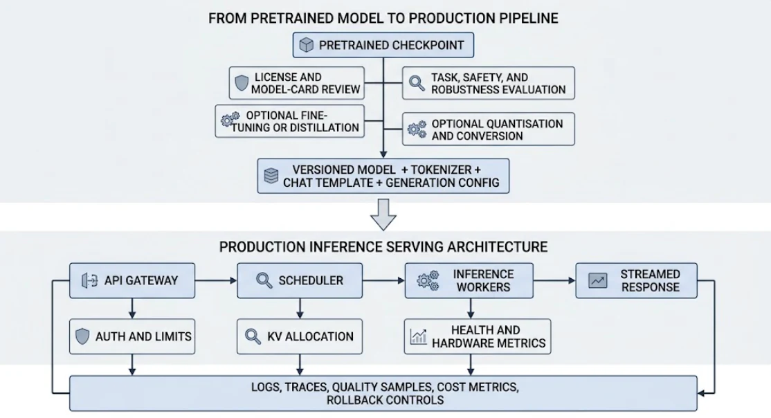
Ultimately, exposing a raw model checkpoint to the internet does not constitute a production service. To guarantee consistent, reliable behavior at scale, a release must be treated as a fully reproducible artifact. This requires locking down every moving part of the execution pipeline: not just the model weights, but the tokenizer version, chat templates, quantization schemes, the specific serving engine, hardware kernels, and generation hyperparameters.
Before routing live traffic to an endpoint, the infrastructure must be rigorously validated against the unpredictable realities of production environments. A robust serving layer must account for:
- Operational resilience: Managing cold-start warm-ups, absorbing massive traffic spikes without crashing, and executing graceful out-of-memory (OOM) recovery when the KV cache fills up.
- Edge cases and client volatility: Handling malformed requests, gracefully truncating prompts that exceed the maximum context window, and safely halting compute when a client rapidly disconnects or cancels a request mid-generation.
- Security and execution boundaries: Strictly enforcing structured-output constraints (e.g., guaranteed JSON schema adherence) and maintaining absolute multi-tenant memory isolation to ensure different users' data remains completely separate.nally, your offline evaluation suite must also run against the live, served API.
Finally, a successful deployment requires running your offline evaluation suite directly against the live, served API. Modifying the quantization strategy, updating a GPU kernel, or swapping the serving framework can subtly alter the model's output distribution—even if your core application code remains completely untouched.
The transformer's architecture and the infrastructure serving it are not separate concerns. A model is only as deterministic as the infrastructure serving it.
本文是三部曲的最後一篇。第一篇文章解析純解碼器 Transformer 的核心架構;第二篇文章則從硬體執行層面,說明 KV 快取、FlashAttention 與模型壓縮如何緩解生成迴圈中的記憶體與頻寬瓶頸。本文將進一步討論如何在正式環境中提供 LLM 服務。
模型本身的執行效率,只是正式服務的一部分。單獨生成 token 是演算法與硬體執行問題;面對持續抵達、長度不一且具不同優先順序的請求時,則成為分散式系統問題。
本文將焦點從模型架構移到服務基礎設施,說明如何把模型運算圖轉化為可擴展、能處理大量同時請求的服務。我們將探討動態請求排程、多 GPU 模型部署,以及吞吐量、延遲與硬體成本之間的取捨,最後說明如何以服務等級目標(SLO)定義並驗證正式環境的效能。
本文結構如下:
1. 請求協調:批次處理策略
相較於輸入結構通常較固定的傳統微服務,LLM 推論工作負載具有更明顯的差異性:
- 非同步抵達:使用者與自動化系統會在不同時間傳送提示詞,抵達速率也會隨負載變化。
- 長度不一:某個請求可能只有五個 token,下一個請求卻可能需要處理包含一萬個 token 的文件。
如果 GPU 逐一處理請求,通常難以充分利用平行運算能力。服務引擎因此會將多個獨立請求組成批次;但由於提示詞與輸出長度不同,各請求不會同時完成,因此批次的組成與更新方式會直接影響吞吐量與延遲。
批次處理的演進
在正式環境中,一個批次通常包含來自多位使用者的獨立請求。這些請求會被放入同一組張量運算中平行執行,但彼此的序列邊界不會混淆;每個請求仍各自維護序列狀態、解碼參數與 KV 快取。
| 策略 | 運作機制 | 正式環境的限制 |
|---|---|---|
| 靜態批次處理 | 伺服器等待累積到預先設定的請求數量,將序列填充(padding)至批次中的最長長度,再一起執行。 | 較短的序列必須等待較長序列完成,容易造成資源浪費與延遲上升。 |
| 動態批次處理 | 伺服器會開啟一段短暫的時間視窗(例如 50 毫秒),在執行前先收集陸續抵達的請求成為一個批次。 | 吞吐量有所改善,但批次的成員,仍然只會在請求的邊界處變動。 |
| 連續批次處理 | 排程器嚴格以 token 為單位運作。在每一個迭代步驟中,它都會將已完成的序列排出,並將新的請求拉進目前作用中的批次。 | 需要進階的快取感知記憶體管理(例如 PagedAttention)才能運作。 |
連續批次處理(也就是迭代層級的排程)已成為主流服務引擎的重要能力。完成的序列可以立即離開,等待中的請求則在後續解碼步驟加入,因而減少批次中因序列長度不同造成的閒置。實際的 GPU 使用率與吞吐量提升幅度,仍取決於模型、硬體、提示詞長度分布與排程設定。
時間(迭代步驟)──────────────────────────────────────►

步驟 1:[ 請求 1 | 請求 2 | 請求 3 | 請求 4 ]
步驟 2:[ 請求 1 | 請求 2 | 請求 3 | 請求 5 ]  ← 請求 4 完成,請求 5 立即遞補
步驟 3:[ 請求 1 | 請求 6 | 請求 3 | 請求 5 ]  ← 請求 2 完成,請求 6 立即遞補
步驟 4:[ 請求 1 | 請求 6 | 請求 7 | 請求 5 ]  ← 請求 3 完成,請求 7 立即遞補

結果:完成的序列可立即被替換,減少批次槽位閒置。
進階排程策略
除了核心的批次處理迴圈之外,排程器還必須運用進階策略,在公平性、優先順序與實體記憶體限制之間取得平衡。
處理記憶體耗盡:搶佔
如果進行中的請求產生比預期更長的回應,KV 快取池可能在生成期間耗盡。此時,排程器可以觸發搶佔:暫停部分低優先順序的請求,將其 KV 快取區塊置換到主機記憶體,或直接釋放並在稍後重新計算前綴。待 VRAM 釋出後,再恢復這些請求。具體策略取決於服務引擎與設定。
緩解資源爭用:分塊預填充
當很長的新提示詞抵達時,若一次完成全部預填充,可能延長單次排程迭代,使其他正在解碼的請求出現延遲尖峰。分塊預填充會將提示詞拆成較小片段,把運算分散到多個排程步驟,讓預填充與解碼更公平地共享資源。
繞過運算:前綴感知路由
在多代理(multi-agent)後端或採用大型標準系統提示詞的應用中,許多請求會共用相同前綴。前綴感知路由與前綴快取會盡可能將這些請求導向已保存相同 KV 狀態的服務實例,重複使用已計算的前綴。命中快取時,可以省去共用部分的預填充運算;實際效益則取決於前綴長度、命中率與快取管理策略。
最大化原始吞吐量不一定符合產品目標。較大的批次可能提高裝置使用率,同時也會增加佇列等待時間與每次解碼迭代的耗時。
2. 擴展執行規模:模型平行化
未經壓縮的 700 億參數模型,以 FP16 儲存權重約需 140 GB,無法完整放入單張 80 GB GPU。即使模型權重能夠容納,大型連續批次所需的 KV 快取也可能超過單一加速器容量。此時,就需要將模型或工作負載分散到多個裝置。
這類做法統稱為模型平行化。分散部署可以突破單一裝置的記憶體與運算限制,但也會引入跨裝置通訊成本。
| 技術 | 切分策略 | 主要通訊方式 | 主要使用情境 | 硬體限制 |
|---|---|---|---|---|
| 資料平行 | 整個模型會被複製到不同的 GPU 上;使用者請求則被分配到各自的 GPU 上處理。 | 請求路由;每個 token 所需的模型通訊量極少 | 為能塞進單一 GPU 的模型,擴展原始吞吐量。 | 若模型本身過大,無法解決 VRAM 容量限制的問題。 |
| 張量平行(垂直切分) | 在同一層之內,將個別的權重矩陣(以及注意力 head)切分到多張 GPU 上。 | 每個層邊界都需要進行集體通訊。 | 容納寬度較大的模型,並降低單一請求的延遲。 | 需要超高頻寬的互連技術(例如 NVLink),才能避免延遲尖峰。 |
| 管線平行(水平切分) | 依序切分模型;例如 GPU A 負責第 1–16 層,GPU B 負責第 17–32 層。 | 各階段之間,點對點傳遞中間的激活值。 | 讓極深的模型,得以跨越多個實體伺服器節點。 | 會引入「管線氣泡」(GPU 閒置等待前一階段完成的空檔時間)。 |
| 專家平行 | 專家混合模型(MoE)中,不同的專家,分別存放在不同的 GPU 上。 | token 需以 all-to-all 的方式,路由到正確的專家 GPU | 為龐大的 MoE 架構提供服務。 | 會產生高度複雜、且流量爆發性強的網路路由開銷。 |
| 上下文平行 | 將龐大的提示詞切成多塊,由不同的 GPU 分別處理不同的序列片段。 | 特定於注意力機制的集體通訊。 | 處理極長的上下文視窗(例如 100 萬個以上的 token)。 | 在預填充階段,會產生大量的網路流量。 |
大型部署通常會組合多種平行化方式,例如張量平行、管線平行與資料平行。分散式推論的重要原則是拓撲感知配置:通訊頻繁的張量平行通常應限制在具備高速互連的節點內;通訊頻率較低的管線階段,則較適合跨節點配置。具體設計仍取決於硬體拓撲與服務引擎。(相關基礎方法可參考〈Megatron-LM〉。)
如果增加 GPU 後,token 延遲或吞吐量沒有改善,應先量測集體通訊時間、管線氣泡與互連頻寬飽和度。平行化以額外通訊換取更多記憶體與運算資源,而實體拓撲決定這項取捨是否有效。
3. 核心張力:吞吐量、延遲與成本
在 LLM 服務部署中,若未說明負載與延遲條件,單獨呈現「每秒 token 數」幾乎沒有比較意義。
批次大小是影響推論效能的重要因素之一。把更多請求放入連續批次,通常能提高 GPU 使用率與整體吞吐量;但硬體同時處理更多序列時,單次 token 迭代也可能耗時更久,進而提高 token 間延遲(ITL)。此外,效能還會受到序列長度、KV 快取容量、模型架構與硬體拓撲影響。
因此,衡量效能時,必須明確定義所處的階段、負載狀況,以及量測的視角。
| 指標 | 定義 | 視角 |
|---|---|---|
| 首個 token 生成時間(TTFT) | 從請求抵達,到第一個串流輸出的 token 為止。 | 使用者體驗(等待系統「思考」) |
| token 間延遲(ITL) | 連續串流輸出的 token 之間的間隔。 | 使用者體驗(閱讀速度) |
| 平均每個輸出 token 耗時(TPOT) | 第一個 token 之後的平均生成時間。 | 系統平均值 |
| 端對端延遲 | 從請求抵達,到最後一個生成的 token 為止。 | 總交易時間 |
| 輸入吞吐量 | 每秒處理的提示詞 token 數。 | 系統容量(受限於預填充) |
| 輸出吞吐量 | 每秒完成生成的 token 數。 | 系統容量(受限於解碼) |
| 請求吞吐量 | 每秒完成的請求數。 | 業務容量 |
提高同時請求數通常能改善整體吞吐量,直到記憶體、運算資源、排程器或互連頻寬飽和。另一方面,請求排隊與批次增大也可能使延遲上升。兩者形成柏拉圖前緣(Pareto frontier):不存在適用所有情境的單一最佳設定,部署團隊必須根據產品 SLO,在硬體效率與使用者體驗之間選擇合適的運作點。
有效基準測試的必要條件
正因為存在這種張力,一個有意義的正式環境基準測試,不能只給出單一一個吞吐量數字,而必須明確說明:
- 提示詞與輸出長度的分布情況
- 抵達速率與同時請求數
- 串流與解碼相關設定(例如貪婪解碼或集束搜尋)
- 模型架構、精度與 KV 快取格式
- 硬體拓撲與互連頻寬
- 服務引擎版本與排程器設定
- 延遲的百分位數(例如 p90、p99),而不能只給平均值
當上線中的系統陷入困境時,執行期出現的症狀,就決定了必須採取哪些介入措施:
| 觀察到的症狀 | 可能的瓶頸 | 可能的介入方式 |
|---|---|---|
| token 串流輸出緩慢(ITL 偏高) | 解碼頻寬受限、批次過大,或分散式通訊速度緩慢。 | 限制連續批次的大小、套用 KV 快取量化、評估推測解碼,或檢查互連流量。 |
| p99 的 TTFT 偏高,但平均值尚可接受 | 預填充階段出現嚴重排隊,或隊首阻塞(head-of-line blocking)。 | 實施嚴格的允入控制、公平排程,以及分塊預填充。 |
| 加速器使用率偏低 | 工作量不足,或排程器本身存在間隙開銷。 | 確認連續批次處理已啟用、提高 token 預算,或使用 CUDA graph 擷取。 |
計算真實成本
對於一個固定的部署方案而言,基礎的基礎設施成本相當直接:
不過,分母(每小時輸出 token 數)必須在服務仍符合延遲 SLO 的指定負載下量測。若請求抵達速率超過系統可持續處理的上限,短時間內可能得到較高的吞吐量數字,卻會使佇列與延遲持續增長。
因此,成本評估必須把延遲 SLO 納入條件。完整的應用程式成本還應包含重試、結構化輸出解析失敗,以及模型壓縮或其他最佳化造成品質退化後所增加的人工審查成本。
4. SLO 思維與服務框架
服務等級目標(SLO)會將執行期行為轉化為可量測的服務承諾。「模型速度要快」無法直接驗證;有效的 SLO 必須定義評估的工作負載、延遲指標、門檻、百分位數與量測時間窗。
舉例來說:
對於長度最多 2,000 個 token 的互動式提示詞:
  p95 TTFT <= 800 毫秒
  p95 ITL  <= 60 毫秒
  錯誤率 < 0.5%
以滾動式 30 分鐘時間窗計算
確切的門檻值,完全取決於產品本身。一個有效 SLO 的關鍵要素,是明確定義的工作負載、特定的百分位數、明確的門檻值,以及量測的時間窗。
尾端延遲陷阱
只看平均延遲,很容易掩蓋 LLM 服務中的尾端問題。由於請求長度差異很大,多數使用者可能很快收到回應,少數請求卻因大型預填充工作或隊首阻塞而等待數十秒。
平均值可能仍顯示系統正常,卻無法反映這些使用者的體驗。因此,SRE 需要追蹤 p90、p95 與 p99 等尾端延遲,並針對等待時間最長的請求分析排程、快取與負載問題。
防禦性工程
要達成 SLO,服務必須具備過載保護。GPU 運算資源與 KV 快取容量都有限,因此正式部署需要明確的防護機制,避免異常、超長或惡意請求影響其他使用者:
- 限制上下文長度: 對允許的最大提示詞與輸出長度,設下硬性上限,避免快取被耗盡。
- 允入控制與負載卸除: 套用嚴格的佇列逾時、針對每個租戶執行速率限制,並在服務耗盡其 VRAM 之前,主動回傳
HTTP 429 Too Many Requests。 - 提示詞驗證: 在 API 閘道端,就先拒絕格式錯誤的輸入或不支援的模態,避免它們被分配到加速器的運算資源。
- 流量隔離: 從實體或邏輯層面,將長時間運行的背景批次工作,與對延遲敏感的互動式使用者流量分開。
品質限制:若為了達成較低的 ITL 而採用更激進的量化或調整解碼設定,卻造成事實錯誤或無效 JSON,這項最佳化便不符合產品需求。延遲與吞吐量必須和任務品質、安全性及結構化輸出有效性一併評估。
服務框架
基本的 Python 腳本可以逐 token 執行 LLM,卻無法提供共享正式服務所需的快取管理、連續排程、可觀測性與過載保護。現代服務框架會整合這些能力,並提供針對特定硬體的執行最佳化。
| 框架 | 最適合的場景 | 值得注意的能力 |
|---|---|---|
| vLLM | 通用型、高吞吐量的加速器服務。 | PagedAttention、連續批次處理、前綴快取、量化(AWQ/GPTQ),以及分散式推論。 |
| SGLang | 複雜的多代理後端與結構化工作流程。 | RadixAttention(前綴重用)、結構化 JSON 輸出,以及分離式服務。 |
| TensorRT-LLM | 針對 NVIDIA 硬體深度最佳化的部署。 | 融合 kernel、飛行中批次處理(in-flight batching)、分頁式快取與分散式推論。 |
| llama.cpp | 本地端、邊緣裝置、CPU、Apple Silicon,以及混合裝置的推論。 | GGUF 量化、廣泛的硬體後端支援、輕量化伺服器,以及連續批次處理。 |
(附註:雖然 Hugging Face TGI 仍存在於許多既有的部署環境中,但其目前的文件,已將該專案描述為維護模式,並建議新的架構部署改用 vLLM、SGLang 或 llama.cpp 等引擎。)
框架選擇應根據目標模型、硬體拓撲、結構化解碼需求、維運能力與實際工作負載決定,而不是只依賴單一公開吞吐量基準。
5. 基礎設施與系統設計參考
本節整理模型行為、基礎設施資源、工作負載階段與維運訊號之間的關係,作為正式環境的快速參考。
5.1 正式環境疑難排解
最佳化應從實際觀察到的瓶頸著手。
| 症狀 | 可能的瓶頸 | 可能的介入方式 |
|---|---|---|
| 長提示詞的 TTFT 偏高 | 預填充運算量,或排程佇列 | FlashAttention、分塊預填充、前綴快取、縮減提示詞,或分離式預填充。 |
| token 串流輸出緩慢(ITL 偏高) | 解碼頻寬,或網路通訊 | 縮小連續批次、權重量化、改用具備 GQA 的模型、推測解碼,或拓撲感知的平行化。 |
| 快取記憶體不足或同時請求數過低 | KV 快取容量 | 分頁式快取管理、採用較少 KV head 的模型、縮短上下文限制、KV 量化,或增加裝置記憶體。 |
| p99 偏高,但平均值尚可接受 | 排隊,或隊首阻塞 | 允入控制、嚴格的流量分級、公平排程,以及分塊預填充。 |
| 加速器使用率偏低 | 工作量不足,或排程間隙 | 確認連續批次處理已啟用、提高 token 預算、使用 CUDA graph 擷取,或調校排程器。 |
| 品質衰退 | 壓縮或解碼方式的變動 | 還原至較高精度、改善校準資料、降低採樣變異度,並執行任務層級的評估。 |
5.2 基礎設施記憶體容量
| 元件 | 硬體概估 |
|---|---|
| 模型權重 | 參數量 每個參數所佔的儲存位元組數 |
| KV 快取 | |
| 訓練梯度 | 參數量 每個梯度所佔的位元組數 |
| 最佳化器狀態 | 依最佳化器而定;通常每個參數對應多個數值 |
| 激活值 | 高度取決於架構、批次大小、序列長度、checkpointing 機制,以及特定的 kernel |
5.3 工作負載階段
| 階段 | 主要工作單位 | 持續性狀態 | 常見瓶頸 |
|---|---|---|---|
| 預訓練 | 完整的訓練批次 | 參數與最佳化器 | 運算、通訊、激活值記憶體 |
| 預填充 | 提示詞或提示詞區塊 | 寫入 KV 快取 | 運算與注意力 IO |
| 解碼 | 每個作用中序列的一個位置 | 讀取並擴充 KV 快取 | 權重/KV 記憶體頻寬與排程 |
5.4 正式環境監控
監控工作,必須把需求、排程器行為、快取壓力、硬體飽和度、使用者可見的延遲,以及模型品質全部連結起來。沒有任何單一指標,能單獨解釋整個系統的狀況。
| 監控層級 | 核心訊號 | 有助於回答什麼問題 |
|---|---|---|
| 需求與工作負載 | 抵達速率、同時請求數、佇列深度、提示詞/輸出分布。 | 整體流量或請求型態是否正在改變? |
| 使用者可見的延遲 | p50、p95、p99 的 TTFT、ITL、TPOT,以及端對端延遲。 | 是哪個推論階段,正在損害使用者體驗? |
| 吞吐量與排程 | 每秒輸入/輸出 token 數、每秒請求數、作用中序列數、每次迭代批次處理的 token 數。 | 排程器是否讓加速器持續有效地忙碌運作? |
| KV 快取健康狀態 | 使用率、配置失敗次數、搶佔次數、驅逐次數、已置換的區塊數,以及前綴快取命中率。 | 快取壓力是否正在限制同時請求數,或導致延遲尖峰? |
| 加速器與網路 | 運算使用率、VRAM 使用量、記憶體頻寬、功耗、溫度,以及互連流量。 | 硬體瓶頸的根源,究竟是運算、記憶體,還是網路? |
| 可靠性 | 取消次數、逾時次數、過載回應(429)、OOM 事件、重啟次數,以及錯誤率。 | 服務是否正安全地卸除或妥善處理失敗的工作? |
| 模型與應用程式品質 | 任務成功率、安全性違規、結構化輸出的有效性、重試次數,以及人工審核比例。 | 某項基礎設施最佳化是否損害了模型原有的任務表現? |
指標應依模型版本、服務設定、工作負載類別與流量優先順序分組。除了平均值,也要使用直方圖與百分位數;告警則應涵蓋 SLO 錯誤預算消耗速率、佇列飽和度等領先指標。任何效能變化都應與品質評估結果交叉檢查。
6. 結語
至此,完整的依賴關係已經清楚呈現:因果注意力會產生可重複使用的 Key 與 Value;張量形狀決定 KV 快取容量;快取隨序列增長,促使服務引擎採用分頁式配置與連續批次排程;正式環境監控則協助團隊找出必須調整的資源或策略,以達成 SLO。
將模型檢查點直接置於 API 之後,並不等於完成正式服務。若要在規模化部署下維持一致性與可靠性,每次發布都必須是可重現的產物。除了模型權重,還要固定 tokenizer 版本、聊天範本、量化方案、服務引擎、硬體 kernel 與生成參數。
在將線上流量導向某個端點之前,基礎設施必須先經過嚴格驗證,以應對正式環境中各種難以預測的現實狀況。一個穩健的服務層,必須考量到:
- 維運韌性: 管理冷啟動與預熱、處理流量尖峰,並在 KV 快取接近容量上限或發生 OOM 時進行復原。
- 邊界情況與使用者端中斷: 處理格式錯誤的請求、依明確政策拒絕或截斷超出上下文上限的提示詞,並在使用者端斷線或取消請求時安全中止運算。
- 安全性與執行邊界: 驗證結構化輸出(例如 JSON schema),並維持多租戶記憶體隔離,避免不同使用者的資料互相暴露。
最後,部署驗證應直接針對實際提供服務的 API 執行離線評估套件。調整量化策略、更新 GPU kernel 或更換服務框架,都可能改變模型輸出分布,即使核心應用程式碼沒有變動。
Transformer 架構與服務基礎設施並非彼此獨立。模型在正式環境中的可預測性與可靠性,取決於整套執行、排程、版本管理與監控機制。