Demand Forecasting with Deep Learning: Does an LSTM Earn Its Complexity?深度學習需求預測:LSTM 值得增加的複雜度嗎?
A practical comparison of a global LSTM with XGBoost across 120 store–SKU series, asking whether learned temporal representations justify the added complexity.以 120 條門市-SKU 序列比較全域 LSTM 與 XGBoost,評估學習式時間表徵能否帶來足以抵銷額外成本的預測改善。
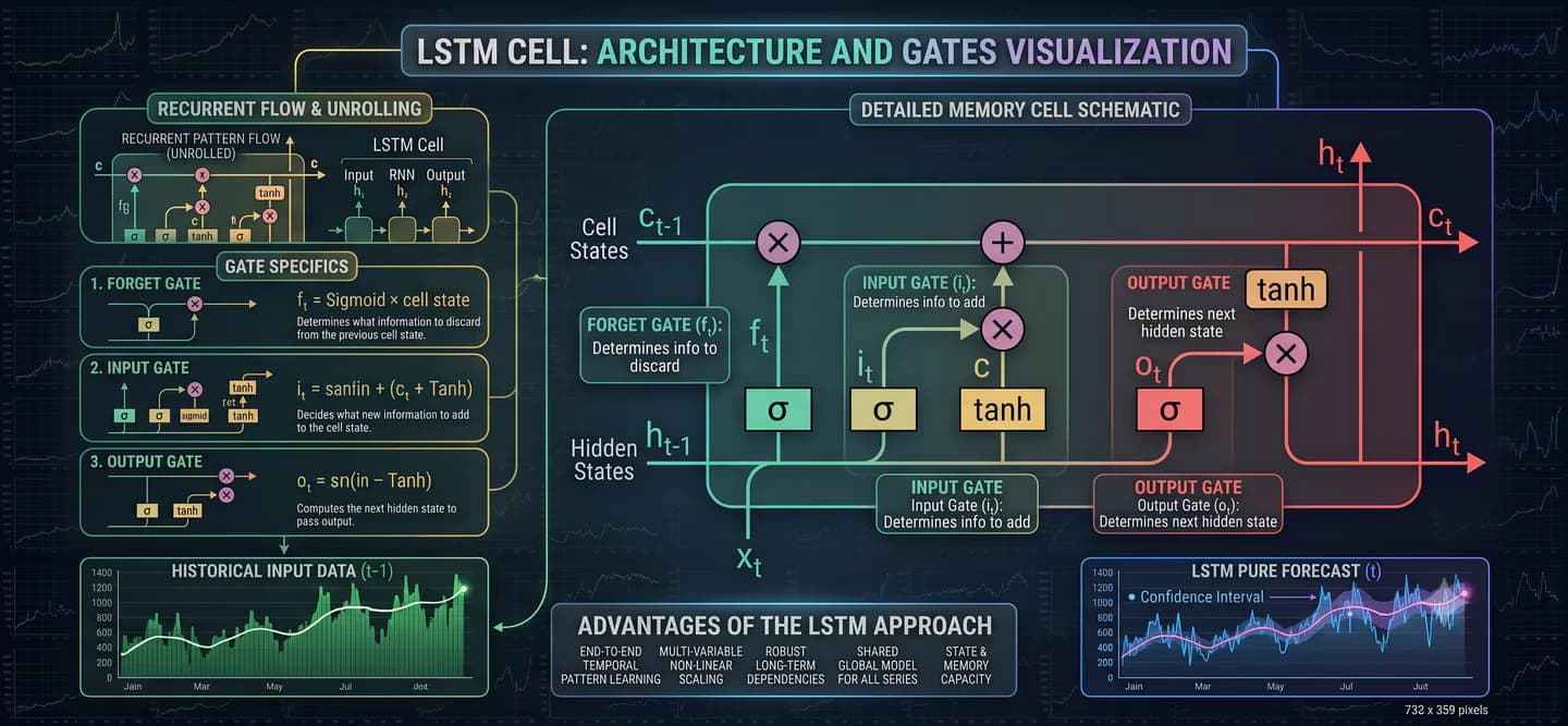
This article continues the case study introduced in:
- Forecasting iPhone 17 Pro Demand: From Statistics to Deep Learning,
- Demand Forecasting with Statistical Models: How Far Can Demand History Alone Take Us?,
- Demand Forecasting with Supervised Learning: Does More Context Help?.
Statistical models provided a strong baseline for one store–SKU, while a global XGBoost scaled forecasting to 120 series but gained little from additional business context. We now test whether a global LSTM can learn directly from ordered demand sequences and improve enough to justify its complexity.
This article is structured as follows:
- Why move beyond engineered features?
- From engineered rows to ordered sequences
- How an LSTM creates memory
- Architecture Design
- Training choices
- Does the improvement justify the complexity?
- Operational recommendation
- Conclusion: complexity must earn its cost
Why move beyond engineered features?
Tabular supervised-learning models such as XGBoost do not receive demand
history as an ordered sequence. We must first convert that history into
features such as lag_7, lag_28, rolling_mean_7, and
rolling_std_28. These features give the model a form of memory, but they
also determine what information that memory contains.
This creates several limitations:
- The temporal representation is predefined. A seven-day lag tells the model to examine the same weekday last week because we decided that relationship was important.
- Historical detail is compressed. A 28-day mean summarises an entire month with one number, potentially hiding the order and shape of changes within that period.
- Longer relationships require more engineering. Extending memory means creating, validating, and maintaining additional lag, rolling, trend, and interaction features.
- A fixed feature set may not capture every series equally well. One product may respond to the previous weekend, while another may depend on a gradual multi-week change that the selected summaries do not preserve.
- More temporal features increase maintenance. Every additional lag, rolling statistic, and interaction must be defined, validated, and reproduced consistently during training and forecasting.
These limitations motivate a different question:
Can a global sequence model learn a shared, nonlinear representation of demand history without relying on predefined statistical structures or handcrafted temporal summaries?
From engineered rows to ordered sequences
A Long Short-Term Memory network, or LSTM, reads the previous demand observations in order. As it moves through the sequence, it updates an internal memory that can retain useful patterns and discard less relevant information. The resulting hidden state becomes a learned representation of recent demand.
Like Holt–Winters and ARIMA, an LSTM preserves the order of historical observations. However, statistical models estimate parameters within predefined structures—such as level, trend, seasonality, and linear lag relationships—whereas an LSTM learns a nonlinear hidden representation from data.
An LSTM is still a supervised-learning model: historical inputs are paired with known targets during training. The change is not from supervised to unsupervised learning. It is from tabular supervised learning with engineered memory to sequence-based supervised learning with learned memory.
XGBoost and the LSTM see the same forecasting problem through different data representations.
| XGBoost | LSTM |
|---|---|
| Receives selected lags and rolling statistics | Receives the previous demand observations in order |
| History is represented through selected lag and rolling features | The representation of history is learned from an ordered sequence |
| Each example is one tabular row | Each example contains an ordered sequence |
| Store and SKU are one-hot encoded | Store and SKU use learned embeddings in the global model |
| Day-ahead context is supplied as columns | Day-ahead context is joined to the learned sequence representation |
For a target date , one LSTM training example looks back 28 days:
The first input is the ordered 28-day demand sequence. The vector contains information known for the target date: calendar position, store status, promotion, discount, price ratio, competitor activity, marketing, and weather. The identifiers and represent the store and SKU; the model converts them into learned embeddings.
Applying this transformation to every eligible target date across all 120 store–SKU series creates the global sequence dataset. Each series contributes examples to the same model, while the chronological training, validation, and test boundaries remain unchanged.
| Window | Target days per series | Global sequences |
|---|---|---|
| Training | 590 | 70,800 |
| Validation | 56 | 6,720 |
| Test | 56 | 6,720 |
The shared LSTM therefore learns from 70,800 training sequences rather than the history of only one store–SKU. Its recurrent parameters can capture temporal behaviour shared across the portfolio without maintaining a separate network for every series.
The LSTM therefore does not eliminate feature engineering entirely. Tomorrow's planned promotion or weather forecast cannot be inferred reliably from past demand, so forecast-time context must remain explicit. What changes is how the historical demand signal is represented.
How an LSTM creates memory
A standard recurrent neural network repeatedly updates a hidden state as it reads a sequence. That gives it memory, but gradients can shrink or grow as they pass through many time steps. Learning longer relationships then becomes difficult.
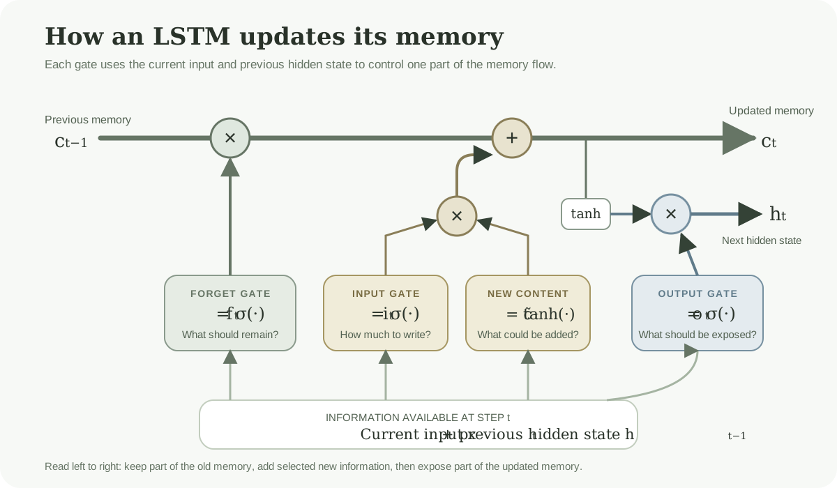
An LSTM introduces a separate cell state and gates that regulate information flow. At day , the model receives the current input , the previous hidden state , and the previous cell state .
The cell state is the LSTM's longer-running internal memory. The hidden state is the exposed representation passed to the next sequence step and, eventually, to the forecasting layers. In the equations below, joins the previous hidden state and current input into one vector. The matrices and vectors are parameters learned during training.
The forget gate decides how much existing memory to retain:
The input gate decides how much new information should be written to memory:
The model separately creates the candidate memory . This is a proposal for what the new information could be, based on the current input and the previous hidden state :
The candidate is not yet the updated cell state. The input gate controls how much of it is added, while the forget gate controls how much of the previous memory remains:
In other words, asks what could be added, decides how much to add, and is the resulting updated memory.
Finally, the output gate controls what memory contributes to the hidden state:
Why sigmoid for gates and tanh for memory?
Sigmoid and tanh perform different jobs inside an LSTM. The sigmoid function produces values between zero and one, making it suitable for controlling how much information passes through a gate. A value near zero blocks information, while a value near one allows most of it through. The forget, input, and output gates therefore use sigmoid as a soft control mechanism rather than an all-or-nothing switch.
The tanh function produces values between and . This allows candidate memory to contain positive or negative internal signals—for example, evidence that the recent demand level is increasing or decreasing. Tanh bounds both the candidate memory and the transformed cell state exposed through ; the internal cell state itself is not restricted to this range.
In short:
Sigmoid controls how much information passes; tanh represents and transforms the information itself.
Why element-wise multiplication?
The symbol represents element-wise multiplication. An LSTM's cell state contains multiple memory components, and each gate produces one control value for every corresponding component. Element-wise multiplication therefore lets the model retain, remove, or expose different parts of its memory independently.
For example, suppose the previous cell state is:
and the forget gate produces:
Then:
Almost all of the first component is retained, 10% of the second remains, and only 1% of the third survives. A dot product would instead collapse these components into one number and prevent component-wise gating.
Element-wise multiplication allows each gate to act like an independent volume control for every component of the LSTM's memory.
In demand forecasting, the cell state might retain a sustained weekly pattern,
reduce the influence of an isolated spike, or update when the recent level
changes for several consecutive days. We do not tell the LSTM to calculate
lag_7 or rolling_mean_28; it learns a hidden representation that is useful
for reducing the forecasting loss.
That flexibility is also a limitation. A hidden state is harder to explain than a named lag or rolling mean, and there is no guarantee that the representation learned from training will remain useful in the next demand regime.
Architecture Design
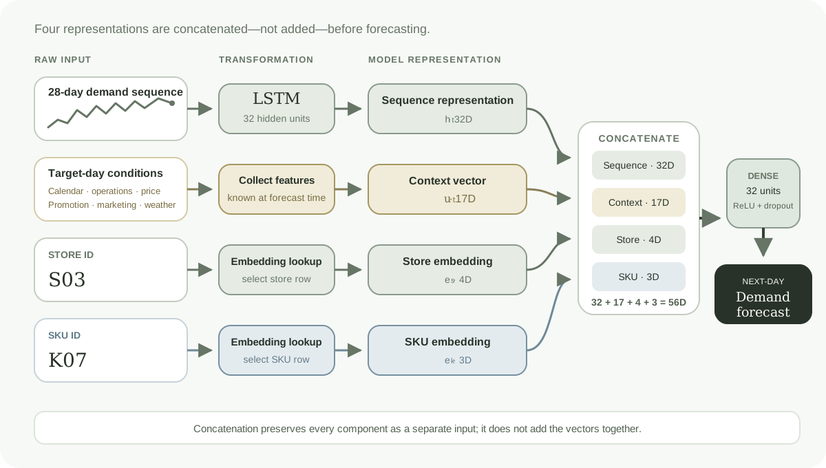
The architecture concatenates four representations rather than adding them numerically:
Here, denotes vector concatenation. The deliberately compact model contains:
- A 28-day demand sequence with one value at each step.
- One LSTM layer with 32 hidden units.
- Seventeen explicit target-day context features.
- Four-dimensional store embeddings and three-dimensional SKU embeddings.
- A dense layer with 32 units, ReLU activation, and 10% dropout.
- One non-negative demand forecast after reversing the scaling transformation.
Together, these components give the global LSTM 6,435 trainable parameters. The objective is not to build the largest neural network, but to test whether a compact learned sequence representation can outperform a strong tabular benchmark.
Building leakage-safe sequences
The experiment retains the same chronological boundaries used in the previous article. The final 112 target dates form consecutive 56-day validation and test windows.
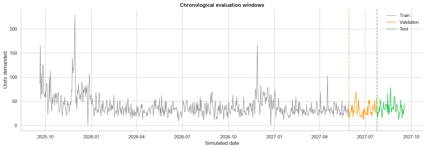
The figure shows one representative series, but the global model applies the same target-date boundaries to all 120 series. Every sample contains the 28 demand observations preceding its target date. The target itself never appears inside the sequence.
LSTM layer setup
The recurrent layer receives only the standardised demand sequence. For a batch containing examples, its input shape is:
The 28 positions represent consecutive historical days, while the final dimension contains one demand value per day. Target-day context and identity embeddings do not enter the recurrent layer; they are added after the sequence has been encoded.
The LSTM layer is configured as:
self.lstm = nn.LSTM(
    input_size=1,
    hidden_size=32,
    batch_first=True,
)
| Setting | Value | Meaning |
|---|---|---|
| Lookback | 28 days | Four weeks of ordered demand history |
| Input size | 1 | One standardised demand value at each step |
| Hidden size | 32 | The hidden and cell states each contain 32 components |
| Batch first | True | Inputs use the shape batch × time × feature |
As the LSTM reads the 28 observations, it updates its hidden and cell states at every step. The implementation keeps only the final hidden state:
_, (hidden_state, cell_state) = self.lstm(sequence)
sequence_representation = hidden_state[-1]
For a batch of sequences, sequence_representation has shape:
This 32-dimensional vector summarises the complete 28-day sequence. The cell state helps maintain memory while the sequence is processed, but it is not passed directly to the forecasting head.
The sequence representation is then concatenated with the 17 target-day context features, four-dimensional store embedding, and three-dimensional SKU embedding:
The resulting 56-dimensional vector enters the dense forecasting network. A single layer with 32 hidden units keeps the architecture deliberately compact: it provides capacity for nonlinear temporal patterns while limiting training cost and overfitting risk.
Learned identity embeddings
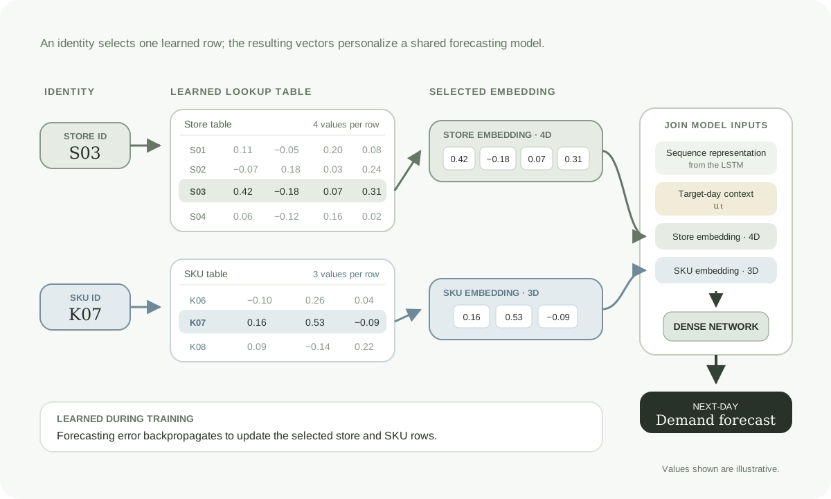
A shared recurrent model can learn temporal behaviour across the portfolio, but it must still distinguish one store or product from another. The same recent demand pattern may imply a different forecast for a high-volume flagship store than for a smaller regional store. The global LSTM handles such differences through learned identity embeddings.
Unlike the XGBoost pipeline, which explicitly one-hot encodes store and SKU identities, the LSTM receives each identity as an integer index.
Store_A → 0
Store_B → 1
Store_C → 2
...
That index directly selects one row from a trainable embedding. An embedding is a learned lookup table: selecting a store or SKU retrieves a small vector of trainable values. In this model, every store receives a four-dimensional vector and every SKU receives a three-dimensional vector
store_embedding = nn.Embedding(
    num_embeddings=n_stores,
    embedding_dim=4,
)
For stores, the model creates a matrix:
The store and SKU vectors are concatenated with the learned sequence representation and target-day business context before entering the dense forecasting layer. The recurrent parameters remain shared across all series, while the embeddings give the downstream network information it can use to make identity-specific adjustments.
Embeddings are updated through backpropagation whenever their store or SKU appears in a training sequence. Identities that require similar forecasting adjustments may develop similar vectors. This does not prove that two stores or products are operationally or economically similar: the vectors encode only what helps reduce the forecasting loss.
Embeddings also create a cold-start limitation. A completely new store or SKU has no learned vector. A production system therefore needs a strategy such as a shared unknown-identity embedding, metadata-based features, or retraining after sufficient history becomes available. Accuracy must still be monitored by series because shared training and embeddings do not guarantee equal performance across the portfolio.
Scaling without future information
Demand levels differ substantially across stores and products. Training one global model on raw units could cause high-volume series to dominate the loss. Therefore, we standardise demand separately for each series:
The mean and standard deviation are calculated using training dates only. Context features are also standardised with a scaler fitted only on the training window. Validation and test data are transformed with those locked statistics.
After prediction, the transformation is reversed to return forecasts to demand units. Negative predictions are clipped to zero because unit demand cannot be negative.
This is an easy place to create leakage. Computing a series mean or standard deviation from all 730 days would allow the future validation and test distributions to influence training. Sequence models do not make point-in-time data discipline less important; they make another preprocessing pipeline that must be protected.
Training choices
After fixing the architecture and input pipeline, three training choices remain especially important: the loss function, gradient control, and the number of training epochs. Together, they determine how the model responds to unusually large errors, how stable each parameter update remains, and how long learning continues before the model begins to overfit the training period.
Huber loss
Daily demand contains occasional large spikes. Squared-error loss gives those
observations rapidly increasing influence, which can encourage the network to
chase unusual events. Huber loss—implemented as SmoothL1Loss—behaves
approximately like squared error near zero and more like absolute error for
large residuals.
The notebook configures and applies it as follows:
LOSS_FUNCTION = nn.SmoothL1Loss(beta=0.5)

prediction = model(sequence, context, store_index, sku_index)
loss = LOSS_FUNCTION(prediction, target)
The beta=0.5 threshold marks the transition from the quadratic to the linear
part of the loss. Because demand is standardised before training, this threshold
is expressed in scaled-demand units.
This does not remove spikes or declare them unimportant. It limits how strongly one extreme residual can dominate an optimisation step.
Gradient Clipping
Training an LSTM requires backpropagation through all 28 sequence steps. Repeated recurrent operations can occasionally produce very large gradients, leading to unstable parameter updates—a problem known as exploding gradients.
After calculating the gradients, the notebook limits their combined norm:
loss.backward()
nn.utils.clip_grad_norm_(
    model.parameters(),
    max_norm=1.0,
)
optimizer.step()
The function calculates the combined Euclidean norm of all model gradients:
If the norm is at most 1, the gradients remain unchanged. If it exceeds 1, all gradients are scaled proportionally:
For example, a total norm of 5 causes every gradient to be multiplied by . This preserves the overall update direction while reducing its magnitude.
Gradient clipping does not alter the model weights, predictions, or loss directly. It limits only the update passed to the optimiser, and it addresses exploding gradients rather than vanishing gradients.
Huber loss and gradient clipping therefore perform complementary roles. Huber loss limits the influence of individual large residuals, while gradient clipping protects the complete optimisation step when the combined gradient becomes unusually large.
The threshold of 1.0 is a training hyperparameter rather than a universal rule. A threshold that is too high may provide little protection, while one that is too low can slow learning. It should therefore be checked through validation and, ideally, gradient-norm monitoring.
Select training duration through validation
Validation loss is checked after every epoch, and training stops after six epochs without improvement. The epoch with the lowest validation loss is locked before the test window is opened.
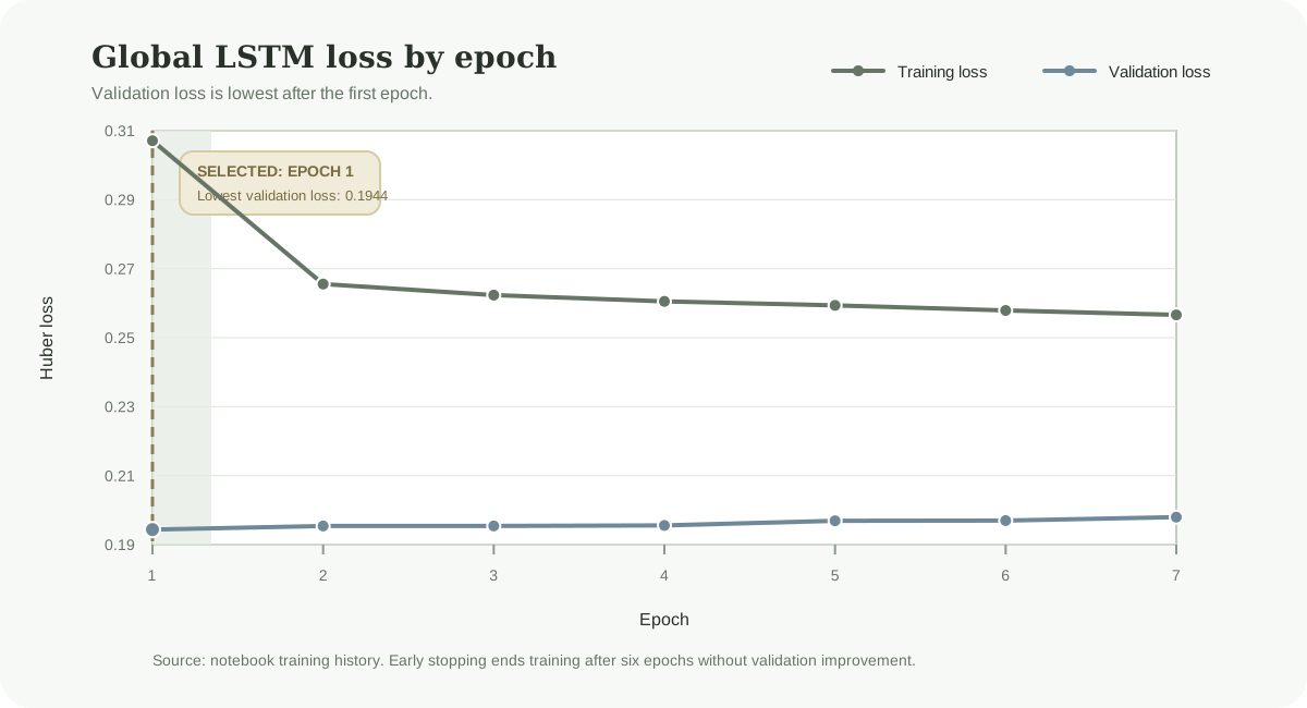
Validation selects only one training epoch for the global LSTM. After that point, training loss continues to fall while validation loss gradually rises. More optimisation improves the fit to the training period but makes the model less useful for the next temporal regime. That is a textbook form of temporal overfitting.
The result is a useful reminder:
Lower training loss does not mean better forecasting of the future.
Early stopping acts as regularisation by limiting how long the model can adapt to training-specific structure. The selected epoch count is not a universal property of LSTMs; it belongs to this architecture, dataset, optimiser, and validation period.
After model selection, a fresh global model is initialised and trained on 77,520 development sequences—the combined training and validation windows—for the single locked epoch. This gives the final model access to every target available before the test boundary. The untouched test window still contributes no information to training duration or model fitting.
Does the improvement justify the complexity?
Deep learning earns its place only if learned temporal representations improve held-out forecasting enough to justify its cost.
Model Comparison
The primary comparison is global LSTM against the global supervised-learning models from the previous article. All results aggregate the same 6,720 test rows across 120 store–SKU series.
This is a comparison of deployable forecasting systems rather than a controlled experiment that changes only the temporal representation. The LSTM also uses a different loss, learned identity embeddings, and a sequence-specific preprocessing pipeline. The result tells us which complete system forecasted better in this holdout; it does not isolate the causal effect of learned memory alone.
| Global model | MAE | RMSE | WAPE | Bias |
|---|---|---|---|---|
| Global LSTM | 5.01 | 6.51 | 26.44% | −2.58% |
| XGBoost: history, calendar, and identity | 5.04 | 6.64 | 26.60% | −4.91% |
| XGBoost: full business context | 5.04 | 6.48 | 26.62% | 2.30% |
| Linear regression: full context | 5.15 | 6.64 | 27.17% | −1.51% |
Global LSTM achieves the lowest WAPE at 26.44%, improving on the strongest XGBoost result by approximately 0.17 percentage points. It also records the lowest MAE, while full-context XGBoost retains the lowest RMSE.
The result supports a narrow conclusion: learned sequence representations are competitive and slightly better on the article's primary metric. It does not support the stronger conclusion that deep learning decisively replaces tabular forecasting. A 0.17-point difference from one 56-day window is too small to separate durable improvement from regime-specific variation without additional rolling evaluation.
Model selection
Model selection is not only an accuracy ranking.
| Consideration | XGBoost | Global LSTM |
|---|---|---|
| Temporal representation | Engineered lags and rolling statistics | Learned from the ordered sequence |
| Training | Fast and comparatively stable | Slower and more sensitive to optimisation choices |
| Identity handling | One-hot encoded fields | Learned embeddings |
| Interpretation | Split importance and tree-based explanations | Hidden states and embeddings require attribution tooling |
| Production data | Feature table | Sequence window, context vector, identities, and locked scalers |
| Overfitting control | Regularisation and early stopping | Dropout, robust loss, and early stopping |
| Prediction intervals | Additional method required | Additional method required |
In this CPU experiment, global-LSTM model selection takes roughly 14 seconds, compared with about one second for XGBoost. The absolute times are small, but the relative difference signals additional cost when tuning expands across architectures, lookback windows, random seeds, and rolling validation periods.
The LSTM removes handcrafted lag and rolling features, but it does not remove the forecasting pipeline. Production must still maintain:
- a correctly ordered 28-day window for every series;
- training-only demand and context scalers;
- store and SKU identity mappings;
- point-in-time business context;
- model weights, embedding tables, and architecture versions;
- monitoring for drift, unstable training, and forecast bias.
Neither model automatically produces calibrated uncertainty. Quantile loss, conformal calibration, or a probabilistic forecasting model would be required before prediction intervals could support service levels or safety stock.
Operational recommendation
Keep history, calendar, and identity XGBoost as the production benchmark and run the global LSTM as a challenger. The LSTM's 0.17-percentage-point WAPE advantage is promising, but it is not enough evidence for an immediate replacement.
Before promoting the LSTM:
- repeat the comparison across additional rolling validation and test windows;
- test multiple random seeds to measure training variability;
- translate forecast differences into stockouts, excess inventory, and service levels;
- monitor bias at panel, store, SKU, and store–SKU levels;
- verify that the sequence and context pipeline can be reproduced reliably;
- add calibrated uncertainty if forecasts will determine safety stock.
In a daily workflow, the trained weights can remain frozen while each series' 28-day demand window and target-day context are refreshed. Weight retraining can happen on a slower schedule and should be triggered by a defined calendar or drift rule rather than by every new observation.
The global model should produce one demand forecast for every store–SKU. Those forecasts are not order quantities. Replenishment still needs stock on hand, confirmed inbound inventory, lead time, pack sizes, service targets, and a chosen uncertainty buffer.
Conclusion: complexity must earn its cost
The progression from XGBoost to LSTM is not simply a move from an old algorithm to a newer one. It changes how the model represents time.
- Tabular supervised learning receives engineered temporal summaries.
- The LSTM receives an ordered sequence and learns a hidden representation.
- Global training supplies enough related sequences for representation learning to become plausible.
- Embeddings let one model share parameters while adjusting for store and SKU.
- Early stopping remains essential because additional optimisation can reduce future accuracy.
The global LSTM wins the panel WAPE table by a narrow margin. Whether it wins the forecasting system depends on what that margin is worth.
For this case study, the honest answer is that deep learning has become competitive, not indispensable. XGBoost remains the benchmark to beat, while the LSTM must prove that its learned memory creates stable operational value across more than one held-out window.
這篇文章延續了以下文章中介紹的案例研究:
統計模型為單一門市-SKU 建立了具競爭力的基準;全域 XGBoost 則將預測擴展到 120 條序列,但額外商業情境資訊帶來的改善有限。本文進一步測試全域 LSTM 能否直接從有序需求序列學習,並產生足以支持其額外複雜度的改善。
本文架構如下:
1. 為什麼要超越人工設計的時間特徵?
像 XGBoost 這類表格型監督式模型,不會直接以有序序列接收需求歷史。建模者必須先將歷史轉換為 lag_7、lag_28、rolling_mean_7 與
rolling_std_28 等欄位。這些特徵為模型提供時間資訊,也同時限制了模型能看見的歷史結構。
這會帶來幾項限制:
- 時間表徵由建模者預先定義。 使用七天落後特徵,代表建模者事先假設上週同一個星期幾具有預測價值。
- 歷史細節被壓縮了。 一個 28 天的平均數,用單一數字概括了整整一個月,可能因此隱藏了這段期間內變化的順序與樣貌。
- 更長期的關係,需要更多工程設計。 延伸記憶,意味著必須建立、驗證並維護更多的落後、滾動、趨勢與交互作用特徵。
- 固定的特徵集合,未必能同等有效地捕捉每一條序列。 某項產品,可能對上一個週末有反應;另一項產品,則可能取決於一個逐漸發生的多週變化,而所選的摘要統計量,並沒有保留這種變化。
- 更多的時間特徵,會增加維護負擔。 每多一個落後特徵、滾動統計量或交互作用,都必須在訓練與預測時,被定義、驗證,並以一致的方式重現。
這些限制,帶出了一個不同的問題:
全域序列模型能否減少對預先定義統計結構與人工時間摘要的依賴,直接學習共享、非線性的需求歷史表徵?
2. 從人工特徵資料列到有序序列
長短期記憶網路(Long Short-Term Memory,LSTM)會依序讀取過去的需求觀測值,並在每個時間步更新內部狀態。最後的隱藏狀態可視為模型從近期需求中學到的序列表徵。
和 Holt-Winters 與 ARIMA 一樣,LSTM 保留了歷史觀測值的順序。不過,統計模型是在預先定義好的結構——例如水準、趨勢、季節性與線性落後關係——之中估計參數,而 LSTM 則是從資料中,學習一個非線性的隱藏表徵。
LSTM 仍然是一種監督式學習模型:在訓練過程中,歷史輸入會與已知的目標值配對。這裡的轉變,並不是從監督式學習變成非監督式學習,而是從 具有工程設計記憶的表格型監督式學習,轉變為 具有學習記憶的序列型監督式學習。
XGBoost 與 LSTM,是透過不同的資料表徵,來看待同一個預測問題。
| XGBoost | LSTM |
|---|---|
| 接收選定的落後特徵與滾動統計量 | 依照順序接收過去的需求觀測值 |
| 透過選定的落後與滾動特徵來表示歷史 | 歷史的表徵,是從有序序列中學習出來的 |
| 每一筆樣本是一列表格資料 | 每一筆樣本包含一段有序序列 |
| 門市與 SKU 經過 one-hot 編碼 | 門市與 SKU 在全域模型中,使用學習到的嵌入向量 |
| 隔日情境資訊以欄位形式提供 | 隔日情境資訊,會與學習到的序列表徵結合 |
對於目標日期 ,一筆 LSTM 訓練樣本,會回顧過去 28 天:
第一個輸入,是有序的 28 天需求序列。向量 ,則包含目標日期已知的資訊:日曆位置、門市營業狀態、促銷、折扣、價格比率、競爭對手動態、行銷與天氣。識別碼 與 ,分別代表門市與 SKU;模型會把它們轉換成學習到的嵌入向量。
把這個轉換,套用到全部 120 條門市-SKU 序列中,每一個符合條件的目標日期上,就建立出了全域序列資料集。每條序列,都為同一個模型貢獻樣本,而依時間順序劃分的訓練、驗證與測試邊界,則維持不變。
| 區間 | 每條序列的目標天數 | 全域序列數 |
|---|---|---|
| 訓練集 | 590 | 70,800 |
| 驗證集 | 56 | 6,720 |
| 測試集 | 56 | 6,720 |
共享 LSTM 會從 70,800 筆訓練序列中學習,而不是只依賴單一門市-SKU 的歷史。循環參數在所有序列之間共享,使模型能捕捉跨門市與產品的共同時間模式,不必為每條序列維護獨立網路。
LSTM 不會完全消除特徵工程。已排定的促銷與天氣預報無法可靠地只從歷史需求推得,因此預測時點的情境資訊仍須明確提供。改變的是歷史需求訊號的表示方式,而不是整個資料管線。
3. LSTM 如何建立記憶
標準的循環神經網路,在讀取序列的過程中,會反覆更新一個隱藏狀態。這讓它具備記憶,但梯度在經過許多時間步之後,可能會縮小或放大,使得學習較長期的關係變得困難。
LSTM 引入了一個獨立的細胞狀態,以及一組用來調節資訊流動的閘門。在第 天,模型接收目前的輸入 、前一個隱藏狀態 ,以及前一個細胞狀態 。
細胞狀態 ,是 LSTM 較長期運作的內部記憶;隱藏狀態 ,則是傳遞給下一個序列步驟、最終再傳遞給預測層的外顯表徵。在以下的方程式中, 把前一個隱藏狀態與目前輸入,結合成一個向量。矩陣 與向量 ,則是訓練過程中學到的參數。
遺忘閘 決定要保留多少既有的記憶:
輸入閘 決定應該把多少新資訊寫入記憶:
模型也會建立候選記憶 ,表示根據目前輸入 與前一個隱藏狀態 所產生的新內容:
這個候選值,還不是更新後的細胞狀態。輸入閘 ,控制要加入多少候選值;遺忘閘 ,則控制要保留多少先前的記憶:
換句話說, 問的是 可以加入什麼, 決定 要加入多少,而 則是最終更新後的記憶。
最後,輸出閘 控制哪些記憶,會貢獻到隱藏狀態之中:
為什麼閘門用 sigmoid,記憶用 tanh?
Sigmoid 與 tanh,在 LSTM 內部扮演不同的角色。Sigmoid 函數,會產生介於 0 到 1 之間的數值,適合用來控制有多少資訊能通過一道閘門:數值接近 0 會阻擋資訊,接近 1 則會讓大部分資訊通過。因此,遺忘閘、輸入閘與輸出閘,都使用 sigmoid 作為一種柔性的控制機制,而不是全有或全無的開關。
Tanh 函數,會產生介於 到 之間的數值。這讓候選記憶,可以包含正向或負向的內部訊號——例如,近期需求水準正在上升或下降的證據。Tanh 會限制候選記憶,以及透過 外顯出來的轉換後細胞狀態;但內部的細胞狀態 本身,並不受限於這個範圍。
簡而言之:
Sigmoid 控制有多少資訊能通過;tanh 則表示並轉換資訊本身。
為什麼使用逐元素相乘?
符號 代表逐元素相乘。LSTM 的細胞狀態,包含多個記憶成分,而每一道閘門,都會為每一個對應的成分,產生一個控制值。因此,逐元素相乘,讓模型能夠獨立地保留、移除,或顯露記憶中的不同部分。
舉例來說,假設前一個細胞狀態是:
而遺忘閘產生的結果是:
那麼:
第一個成分幾乎完全保留、第二個成分保留了 10%、第三個成分則只剩下 1%。如果改用內積,這些成分就會被壓縮成單一一個數字,導致無法逐成分進行閘控。
逐元素相乘讓閘門可以分別控制記憶向量中的不同成分。
在需求預測中,細胞狀態可能會保留一個持續存在的每週模式、降低某次孤立尖峰的影響力,或是在近期水準連續好幾天發生變化時進行更新。我們並不會告訴 LSTM 去計算 lag_7 或 rolling_mean_28;它學到的,是一個有助於降低預測損失的隱藏表徵。
這種彈性,同時也是一種限制。隱藏狀態,比一個有名稱的落後特徵或滾動平均,更難以解釋;而且,也無法保證訓練中學到的表徵,在下一個需求狀態中,依然有用。
4. 架構設計
這個架構會串接四種表徵,而不是直接逐元素相加:
其中, 代表向量串接。這個刻意保持精簡的模型包含:
- 一段 28 天的需求序列,每一步一個數值。
- 一層具有 32 個隱藏單元的 LSTM 層。
- 17 個明確的目標日情境特徵。
- 四維的門市嵌入向量,以及三維的 SKU 嵌入向量。
- 一層具有 32 個單元、ReLU 啟動函數與 10% dropout 的密集層。
- 還原縮放轉換後,得到一個非負的需求預測值。
整體全域 LSTM 共有 6,435 個可訓練參數。實驗目的不是建立大型網路,而是測試精簡的學習式序列表徵能否優於具競爭力的表格型基準。
建立防止洩漏的序列
這項實驗,沿用了前一篇文章所使用的時間邊界。最後 112 個目標日期,構成連續的 56 天驗證區間與 56 天測試區間。
這張圖顯示的是一條具代表性的序列,但全域模型,會把相同的目標日期邊界,套用到全部 120 條序列上。每一筆樣本,都包含目標日期之前的 28 筆需求觀測值;目標值本身,絕不會出現在序列之中。
LSTM 層的設定
循環層,只會接收標準化後的需求序列。對於包含 筆樣本的一個批次,它的輸入形狀為:
這 28 個位置,代表連續的歷史天數;最後一個維度,則包含每天的一個需求值。目標日情境資訊與身分嵌入向量,並不會進入循環層,而是在序列被編碼之後才加入。
LSTM 層的設定如下:
self.lstm = nn.LSTM(
    input_size=1,
    hidden_size=32,
    batch_first=True,
)
| 設定 | 數值 | 意義 |
| 回顧期間 | 28 天 | 四週的有序需求歷史 |
| 輸入維度 | 1 | 每一步一個標準化後的需求值 |
| 隱藏維度 | 32 | 隱藏狀態與細胞狀態,各包含 32 個成分 |
| Batch first | True | 輸入的形狀為 batch × time × feature |
當 LSTM 讀取這 28 筆觀測值時,會在每一步更新它的隱藏狀態與細胞狀態。這個實作,只保留最後一個隱藏狀態:
_, (hidden_state, cell_state) = self.lstm(sequence)
sequence_representation = hidden_state[-1]
對於一個包含 段序列的批次,sequence_representation 的形狀為:
這個 32 維向量,概括了整段 28 天的序列。細胞狀態,有助於在處理序列的過程中維持記憶,但並不會直接傳遞給預測輸出層。
接著,這個序列表徵,會與 17 個目標日情境特徵、四維的門市嵌入向量,以及三維的 SKU 嵌入向量串接在一起:
得到的 56 維向量會進入密集預測網路。單層、32 個隱藏單元的設計刻意保持精簡,在提供非線性建模能力的同時控制訓練成本與過度配適風險。
學習到的身分嵌入
一個共享的循環模型,能夠學習整個商品組合中的時間行為,但仍然必須區分不同的門市或產品。同樣的近期需求模式,對一家高銷量的旗艦門市,與一家較小的區域門市而言,可能意味著不同的預測結果。全域 LSTM,透過學習到的身分嵌入向量,來處理這類差異。
與明確使用 one-hot 編碼門市與 SKU 身分的 XGBoost 流程不同,LSTM 接收到的每一個身分,都是一個整數索引。
Store_A → 0
Store_B → 1
Store_C → 2
...
這個索引,會直接從一個可訓練的嵌入表中,選出對應的一列。 嵌入向量,是一種學習到的查找表:選取一個門市或 SKU,就會取出一小組可訓練數值所組成的向量。 在這個模型中,每一家門市,會得到一個四維向量;每一個 SKU,則會得到一個三維向量
store_embedding = nn.Embedding(
    num_embeddings=n_stores,
    embedding_dim=4,
)
對於 家門市,模型會建立一個矩陣:
門市與 SKU 向量,會在進入密集預測層之前,與學習到的序列表徵及目標日商業情境串接在一起。循環參數,在所有序列之間維持共享;而嵌入向量,則為下游網路提供了可用來做出身分專屬調整的資訊。
每當某個門市或 SKU 出現在訓練序列中,它對應的嵌入向量,就會透過反向傳播進行更新。需要類似預測調整的身分,可能會演變出相似的向量。但這並不能證明兩家門市或兩項產品,在營運或經濟意義上是相似的——這些向量,編碼的只是有助於降低預測損失的資訊。
嵌入向量也會造成冷啟動限制:全新門市或 SKU 沒有已學習的向量。正式系統需要預先定義處理方式,例如使用「未知身分」嵌入、加入中繼資料特徵,或在累積足夠歷史後重新訓練。共享訓練與嵌入並不保證所有序列表現一致,因此仍須逐層級監控準確度與偏差。
不使用未來資訊的縮放
不同門市與產品之間的需求水準,差異相當大。如果直接用原始台數,訓練單一全域模型,可能會讓高銷量的序列主導整體損失。因此,我們針對每一條序列,各自進行需求標準化:
平均數 與標準差 ,只用訓練集的日期來計算。情境特徵,也是用只在訓練區間上配適的縮放器來標準化。驗證與測試資料,則使用這些已鎖定的統計量來轉換。
預測完成後,這個轉換會被還原,把預測值換回需求台數。負的預測值會被截斷為零,因為需求台數不可能為負。
這是一個很容易產生洩漏的地方。如果用全部 730 天的資料,來計算一條序列的平均數或標準差,就會讓未來驗證集與測試集的分布,影響到訓練過程。序列模型,並不會讓即時時點的資料紀律變得比較不重要;它們只是多了一條,同樣需要被妥善保護的前處理管線。
5. 訓練設定
固定架構與輸入管線後,三項訓練設定特別重要:損失函數、梯度控制與訓練週期(epoch)數。它們分別影響模型如何處理大型誤差、參數更新的穩定度,以及何時開始對訓練期間過度配適。
Huber 損失
每日需求中,偶爾會出現大幅的尖峰。平方誤差損失,會讓這些觀測值的影響力快速增加,可能因此促使網路去追逐異常事件。Huber 損失——在實作中對應到 SmoothL1Loss——在誤差接近零時,行為近似平方誤差;而在殘差較大時,則更接近絕對誤差。
筆記本中,是這樣設定並套用它的:
LOSS_FUNCTION = nn.SmoothL1Loss(beta=0.5)

prediction = model(sequence, context, store_index, sku_index)
loss = LOSS_FUNCTION(prediction, target)
beta=0.5 這個門檻值,標記出損失函數從二次項過渡到線性項的位置。由於需求在訓練前已經過標準化,這個門檻值,是以縮放後的需求單位來表示的。
這並不會移除尖峰,也不代表尖峰不重要。它限制的,是單一一個極端殘差,能在一次最佳化步驟中,主導到什麼程度。
梯度裁剪
訓練 LSTM 需要沿 28 個序列步驟反向傳播。循環運算可能產生過大的梯度,使參數更新不穩定,這個問題稱為梯度爆炸。
在計算出梯度之後,筆記本會限制它們的合併範數:
loss.backward()
nn.utils.clip_grad_norm_(
    model.parameters(),
    max_norm=1.0,
)
optimizer.step()
這個函式,會計算模型所有梯度合併後的歐幾里得範數:
如果這個範數不超過 1,梯度就會維持不變。如果超過 1,所有梯度都會按比例縮放:
舉例來說,如果總範數是 5,每一個梯度就會被乘上 。這樣可以保留整體更新的方向,同時降低其幅度。
梯度裁剪,並不會直接改變模型權重、預測值或損失。它只限制傳遞給最佳化器的更新量,而且處理的是梯度爆炸,而不是梯度消失。
因此,Huber 損失與梯度裁剪,扮演的是互補的角色。Huber 損失,限制個別大型殘差的影響力;梯度裁剪,則在合併後的梯度異常龐大時,保護整個最佳化步驟。
1.0 是本實驗的超參數,不是通用規則。門檻太高可能無法有效限制梯度,太低則可能減緩學習;應搭配驗證結果與梯度範數監控調整。
透過驗證來選擇訓練時長
每一個訓練週期結束後,都會檢查驗證損失;如果連續六個週期都沒有改善,訓練就會停止。驗證損失最低的那個週期,會在打開測試區間之前先行鎖定。
驗證集,為全域 LSTM 只選出了一個訓練週期。在那之後,訓練損失持續下降,但驗證損失卻逐漸上升。更多的最佳化,改善的是模型對訓練期間的配適程度,卻讓模型對下一個時間狀態變得較不實用。這正是時間性過度配適的典型範例。
這個結果,是一個有用的提醒:
更低的訓練損失,不代表對未來有更好的預測。
提前停止,透過限制模型能適應訓練特定結構的時間長度,發揮了一種正則化的作用。選定的週期數,並不是 LSTM 的普遍性質,而是專屬於這個架構、這份資料集、這個最佳化器與這段驗證期間的結果。
完成模型選擇後,系統會重新初始化全域模型,並在訓練集與驗證集合併後的 77,520 筆開發序列上,依已鎖定的 epoch 數重新訓練。最終模型因此可以使用測試邊界前的所有目標值,而測試區間仍不參與訓練時長選擇或模型配適。
6. 改善幅度是否值得增加複雜度?
只有當學習式時間表徵在未見資料上的改善足以抵銷額外成本時,採用深度學習才具有實務依據。
模型比較
主要的比較,是全域 LSTM 對比前一篇文章中的全域監督式學習模型。所有結果,都是彙總自全部 120 條門市-SKU 序列中,相同的 6,720 列測試資料。
這是完整預測系統之間的比較,不是只替換時間表徵的控制實驗。LSTM 同時採用不同損失函數、身分嵌入與序列專屬前處理。因此,結果只能比較兩套系統在本次測試中的整體表現,不能單獨歸因於學習式記憶。
| 全域模型 | MAE | RMSE | WAPE | 偏差 |
|---|---|---|---|---|
| 全域 LSTM | 5.01 | 6.51 | 26.44% | −2.58% |
| XGBoost:歷史、日曆與身分 | 5.04 | 6.64 | 26.60% | −4.91% |
| XGBoost:完整商業情境 | 5.04 | 6.48 | 26.62% | 2.30% |
| 線性迴歸:完整情境 | 5.15 | 6.64 | 27.17% | −1.51% |
全域 LSTM 的 WAPE 最低,為 26.44%,比最佳 XGBoost 低約 0.17 個百分點。它也取得最低 MAE;完整情境 XGBoost 則有最低 RMSE。
結果支持一項有限結論:學習式序列表徵具有競爭力,並在主要指標上略好。但單一 56 天區間中 0.17 個百分點的差異,不足以證明深度學習可以取代表格型模型;仍需額外滾動評估,判斷改善是否穩定。
模型選擇
模型選擇,不只是替準確度排名而已。
| 考量因素 | XGBoost | 全域 LSTM |
|---|---|---|
| 時間表徵 | 工程設計出來的落後特徵與滾動統計量 | 從有序序列中學習而來 |
| 訓練 | 較快,也相對穩定 | 較慢,且對最佳化選擇較敏感 |
| 身分處理 | One-hot 編碼欄位 | 學習到的嵌入向量 |
| 解讀方式 | 切分重要性與樹狀解釋 | 隱藏狀態與嵌入向量,需要額外的歸因工具 |
| 正式環境所需資料 | 特徵表格 | 序列視窗、情境向量、身分識別碼,以及已鎖定的縮放器 |
| 過度配適控制 | 正則化與提前停止 | Dropout、穩健損失函數與提前停止 |
| 預測區間 | 需要額外的方法 | 需要額外的方法 |
在這個以 CPU 執行的實驗中,全域 LSTM 的模型選擇,大約需要 14 秒,相較之下,XGBoost 只需要大約 1 秒。絕對時間雖然不長,但這個相對差異,預示著當調校範圍擴大到不同架構、回顧視窗、隨機種子與滾動驗證期間時,會帶來額外的成本。
LSTM 減少了人工設計的落後與滾動特徵,但沒有消除預測管線。正式環境仍須維護:
- 每一條序列,都要有正確排序的 28 天視窗;
- 只在訓練集上配適的需求與情境縮放器;
- 門市與 SKU 的身分對照表;
- 即時時點的商業情境;
- 模型權重、嵌入表,以及架構版本;
- 對飄移、不穩定訓練與預測偏差的監控。
這兩種模型,都不會自動產生校準良好的不確定性估計。在預測區間,能夠支援服務水準或安全庫存之前,都需要額外的分位數損失函數、共形校準,或機率預測模型。
7. 營運建議
建議保留「歷史、日曆與身分」XGBoost 作為正式基準,並讓全域 LSTM 以挑戰模型方式並行運作。LSTM 的 WAPE 低 0.17 個百分點,但目前證據不足以支持立即替換。
在將 LSTM 升級為正式模型之前:
- 在更多滾動驗證與測試區間中,重複這項比較;
- 測試多個隨機種子,衡量訓練過程的變異程度;
- 把預測結果的差異,換算成缺貨、庫存過剩與服務水準的實際影響;
- 在全體序列、門市、SKU 與門市-SKU 各個層級,監控偏差;
- 確認序列與情境管線,能夠被可靠地重現;
- 如果預測結果,將用來決定安全庫存,就需要加入校準良好的不確定性估計。
在每日的作業流程中,已訓練好的權重可以維持凍結,只更新每條序列的 28 天需求視窗,以及目標日的情境資訊。權重的重新訓練,可以按照較慢的節奏進行,並且應該由明確定義的行事曆規則,或飄移規則來觸發,而不是每來一筆新的觀測值就重新訓練一次。
全域模型,應該為每一個門市-SKU,產生一個需求預測。這些預測,並不是訂購數量。補貨決策,仍然需要現有庫存、已確認到貨量、前置時間、包裝規格、服務目標,以及所選定的不確定性緩衝。
8. 結論:複雜度必須帶來相稱價值
從 XGBoost 演進到 LSTM,並不只是從一個較舊的演算法,換成一個較新的演算法而已。它改變的,是模型表示時間的方式。
- 表格型監督式學習,接收的是工程設計出來的時間摘要統計量。
- LSTM,接收的是一段有序序列,並學習一個隱藏表徵。
- 全域訓練,提供了足夠多的相關序列,讓表徵學習變得可行。
- 嵌入向量,讓單一模型能共享參數,同時針對門市與 SKU 做出調整。
- 提前停止仍然重要,因為持續降低訓練損失,可能反而損害未見資料上的準確度。
全域 LSTM,以些微的差距,在全體序列彙總的 WAPE 表格中勝出。但它是否能贏得整個預測系統的採用,取決於這個差距究竟值多少。
就本案例而言,深度學習已具競爭力,但尚非必要選擇。XGBoost 仍是需要被穩定超越的基準;LSTM 則必須在多個未見時間區間中,證明學習式記憶能持續創造營運價值。